Nature, Published online: 30 October 2024; doi:10.1038/d41586-024-03392-4
An innovative approach to 3D printing has been developed in which acoustic vibrations and light control the formation of a solid at an air–liquid interface. The strategy enables fast printing of objects with highly detailed features.
Nature, Published online: 29 October 2024; doi:10.1038/d41586-024-03397-z
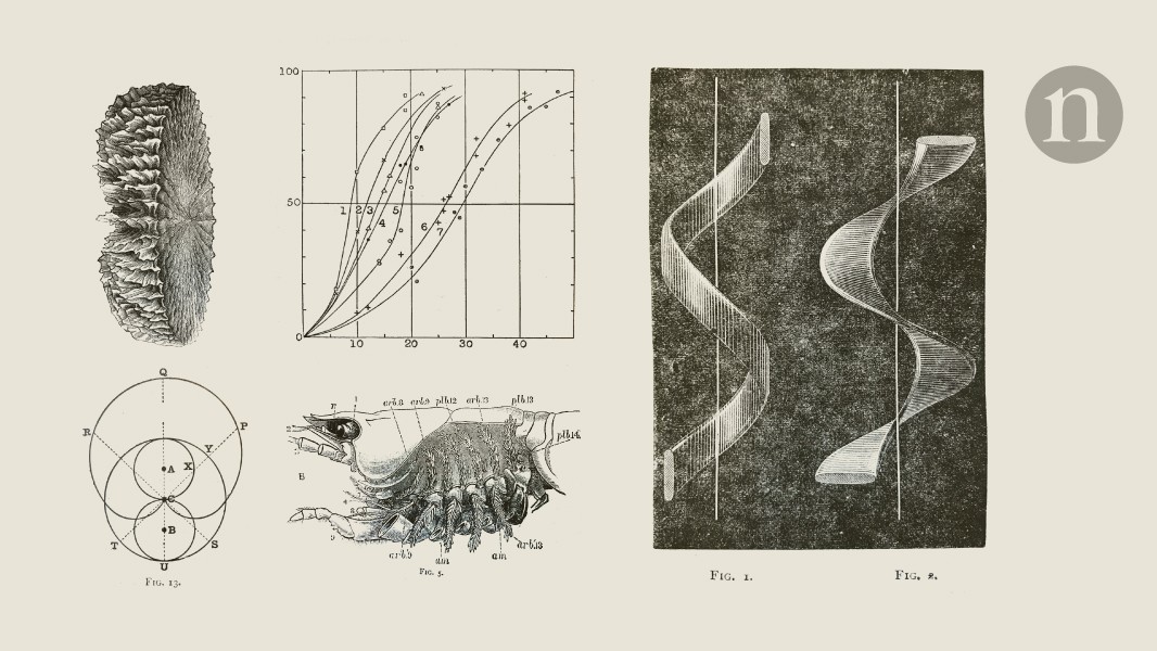
Precise calculations on the erection of Stonehenge’s boulders, and a bright aurora stretches between the stars, in our weekly peek at Nature’s archives.
Thank you for visiting nature.com. You are using a browser version with limited support for CSS. To obtain
the best experience, we recommend you use a more up to date browser (or turn off compatibility mode in
Internet Explorer). In the meantime, to ensure continued support, we are displaying the site without styles
and JavaScript.
Using H2-based redox reactions, our ‘one step oxides to bulk alloy’ operation (Fig. 1a) is aimed to reform the millennia-old multi-step alloy-making process (Fig. 1a, top) in three aspects: first, eliminating CO2 emission during fossil reductant-based metal extraction; second, reducing the energy cost of liquid processing15,16 that scales with melting temperatures; and third, exploiting the diffusion processes involved directly for compaction. The a priori feasibility of our sustainable alloy synthesis route is governed by the thermodynamic nature of the traditionally separated process steps that we merge here: metal extraction from oxides, atomic-scale mixing amongst the alloying elements and bulk material compaction by diffusion. (Fig. 1a, bottom). Our approach is based on a general thermodynamic design treasure map (Fig. 1b), using the two most important physical parameters involved: solid-state reducibility of oxides in H2, as quantified by \(\Delta {G}_{{\rm{oxide}}}-\Delta {G}_{{{\rm{H}}}_{2}{\rm{O}}}\); and alloying capability, as quantified by the mixing enthalpy between substances (we exemplify Fe–X binary systems in Fig. 1b). Elements in the first and the fourth quadrants (Fe, Ni, Co and Cu) are those that can be fully reduced from their oxides at the solid state by H2, and the closer they locate to the ideal mixing line signifies the more preferential substitutional alloying capability with Fe (Fig. 1b). The thermodynamic validity of our design treasure map well aligns with both historical attempts on alloyed powders17 or nano-composite18 fabrication and the more recent literature on H2-based direct oxide reduction19,20,21.
Fig. 1: One-step sustainable synthesis of bulk alloys with defined microstructures from oxides.
a, Schematic comparison between the traditional multi-step alloy-making process and the proposed sustainable ‘one step oxides to bulk alloy’ operation. b, Thermodynamically informed design treasure map. For simplicity, here the reducibility (\(\Delta {G}_{{\rm{oxide}}}-\Delta {G}_{{{\rm{H}}}_{2}{\rm{O}}}\)) is considered for the oxides with the highest valence states at 700 °C under 1 atm. Thermodynamic data for constructing this diagram have been collected from the literature2,41 and the SGTE database42. c, Kinetic conception outlining the two main competing factors in achieving bulk alloys with defined microstructures from oxides, related in part to the present demonstrator Fe–Ni alloy class. The physical rationale of such a proposition lies in the difference between the oxide reduction temperature and the temperature at which complete densification is achieved (typically when T/Tm ≈ 0.75, where Tm is the bulk melting point35; see also Extended Data Fig. 1) in the corresponding metallic phase. The critical heating rate, βc, indicates the scenario in which complete oxides-to-alloy conversion and complete densification are simultaneously achieved. β1 and β2 sketch two heating rates slower than βc as a guide to the eye.
For synthesizing not just powders or nanoparticles, but bulk alloys ready for applications, a secondary consideration promptly emerges: sufficient densification and reproducible bulk properties must be attained, which is governed by the kinetics of the underlying mass transport and microstructure formation mechanisms. This design rationale is essential as conventional multi-step alloy-making always requires a third step to reheat the as-cast materials for thermomechanical processing, endowing them with the desired microstructure–property combinations (Fig. 1a, top). Although a quantitatively precise kinetic design guideline relies on the targeted alloy system and product properties, a general conception could still be made, considering the overall interplay between oxides-to-alloy conversion and densification (Fig. 1c). In a theoretical framework encompassing temperature, time and conversion rate, these two phenomena divide the kinetic processing space into four regions, in which a critical heating rate is also involved: our ‘one step oxides to bulk alloy’ operation may be possible only in regions (i) and (ii) in which oxides-to-alloy conversion finishes before complete densification, and further temperature increase in region (i) leads only to salient microstructural coarsening. Regions (iii) and (iv) conversely suggest an incomplete oxides-to-alloy conversion, with moderate or noticeable densification depending on the temperature, respectively. Bearing these semi-quantitative thermodynamic–kinetic guidelines in mind, we next practise our ‘one step oxides to bulk alloy’ concept, aiming to synthesize bulk green Fe–Ni invar alloys as a demonstration. This endeavour is motivated by the substantial environmental costs2,14 associated with fabricating this class of attractive ferrous materials using the conventional extraction–alloying–thermomechanical processing three-step alloy-making procedure.
Following the thermodynamic design treasure map (Fig. 1b), we first assess all the possible redox reactions in more quantitative depth. As seen in the calculated Ellingham–Richardson diagram, oxides of Fe and Ni with different valence states all locate above the 2H2 + O2 → 2H2O reaction beyond about 600 °C, suggesting the reducibility of these oxides by H2, and thereby, the formation of metallic Fe and Ni far below their melting points (Fig. 2a,b and Extended Data Fig. 1). To achieve an invar alloy, sufficiently homogeneous mixing between Fe and Ni is indispensable, and the extensive single-phase face-centred cubic (fcc) phase field in the Fe–Ni binary system alleviates such a concern: infinite solubility is present for alloys with more than 20 atomic percent (at.%) Ni above 600 °C. We next mixed Fe2O3 and NiO powders using low-energy ball milling (Fig. 2c,d, left), targeting the Fe–Ni ratio in the invar alloy and compacted them into pellets (Fig. 2e). With this precursor material, we mimic a naturally blended ore with all gangue oxides removed, motivating a proof-of-concept exploration. Secondary electron imaging and energy dispersive X-ray spectroscopy (EDS) confirm the homogeneous mixing of the two oxide powders (Fig. 2c) without discernible mechanical alloying.
Fig. 2: Synthesis kinetics, microstructure and thermal expansion property of the invar alloy fabricated from oxides.
a, Minimum melting energy cost as a function of the melting point for common species. The estimation is conducted by adding the enthalpy change of heating up a certain substance from ambient temperature to its melting point and the enthalpy of fusion, that is, \({\Delta E}_{\min }={\int }_{{25}^{^\circ }{\rm{C}}}^{{T}_{{\rm{m}}}}{c}_{{\rm{p}}}\,{\rm{d}}T+{\Delta H}_{{\rm{f}}}\). Only the enthalpy of fusion is considered for ice. Thermophysical parameters for these estimations are acquired from the literature41. b, Predicted Ellingham–Richardson diagram for the oxides of Fe (Fe2O3, Fe3O4 and FeO) and Ni (NiO) under 1 atm (SGTE database42 and refs. 2,41). c, Secondary electron micrograph of the Fe2O3 + NiO powder mixture and the corresponding EDS maps. d, Two-dimensional SXRD diffractograms of the as-compacted oxide pellet (left) and the synthesized invar alloy (right). e, Macroscopic morphological evolution at different conversion rates. f, TGA curve showing the reduction kinetics. Inset: the instantaneous mass loss as a function of time. g, IPF map of the as-synthesized alloy (Σ3 annealing twin boundaries are excluded). h, The corresponding phase map. i, EDS mapping of Fe and Ni. j, Bulk thermal expansion (top, measured using dilatometer) and lattice thermal expansion (bottom, measured using in situ SXRD) results. The bulk and the lattice thermal expansion data for the invar alloys fabricated using different methods are reproduced from the literature25,26,29,30. k, Examples of microstructure tunability. Details of the microstructure after pressure-free sintering are provided in Extended Data Fig. 2. i, Vickers hardness and bulk mass density comparison among the green invar alloys synthesized from oxides and the one fabricated using the conventional melting–casting–recrystallization (REX) method. The recrystallization conditions for the invar alloy processed through melting–casting were also chosen as 900 °C, 0.5 h (around 70% cold-rolling thickness reduction), whose grain size is about 50 μm. a.u., arbitrary units; CTE, coefficient of thermal expansion. Scale bars, 1 μm (c, top and bottom, i); 5 mm (e); 2 μm (g,h); 5 μm (k).
Following the kinetic conception (Fig. 1c), we adopted a moderate heating rate of 5 °C min−1. When heated up in a H2 atmosphere, the pellet undergoes noticeable mass loss accompanied by volumetric shrinkage and colour change (Fig. 2e,f), underpinning the activation of redox reactions. Three stages can be discerned in the thermogravimetric analysis (TGA) (Fig. 2f): (1) reduction initiates at around 290 °C, with a linear increase in conversion rate until an inflection point at about 400 °C, where the reaction is momentarily impeded; (2) the conversion rate resumes to show a linear dependence on temperature in the 450–580 °C range; and (3) an asymptotic trend is present as the conversion rate approaches 0.95 until complete reduction. The presence of distinctive stages in the TGA curve implies the involvement of several redox and alloying micro-events22,23, as rationalized later. At complete reduction, the pellet exhibits a silvery surface, in distinctive contrast with the red-hematite appearance of its as-compacted counterpart (Fig. 2e). Synchrotron X-ray diffraction (SXRD) measurement further validates the single fcc phase constitution of the fully reduced pellet (Fig. 1d, right), in which no remaining oxide phase is detected. The lattice constant of this fcc phase is 3.60 Å. Even considering the uncertainties involved in various measurement techniques, such a lattice constant value agrees well with the literature data for Fe–Ni invar alloys24,25,26 (about 3.60 Å); however, it is notably larger than that of pure fcc-Ni24,27,28 (about 3.52 Å). This distinction evidences substitutional alloying between Fe and Ni during the solid-state redox synthesis, staying consistent with our theoretical anticipation. With this, we prove that the traditionally separate steps of metal extraction and mixing can be merged in a single operation under suitable thermodynamic–kinetic boundary conditions (Fig. 1a).
To assess the ‘oxides to bulk invar alloy’ proposition, we characterize the microstructure and examine the thermal expansion property of the synthesized alloy. Figure 2g shows the electron backscatter diffraction (EBSD) inverse pole figure of the as-synthesized alloy, revealing an equiaxed grain morphology with a fine average grain size of approximately 0.58 μm. Despite the sub-micro-scale porosity owing to the redox-catalysed mass loss and incomplete densification, the microstructure exhibits a single fcc phase constitution (Fig. 2h) without detectable body-centred cubic (bcc) or residual oxide phase at the spatial resolution limit of EBSD (around 50 nm). EDS maps also verify the grain-level uniform distribution of Fe and Ni (Fig. 2i), the contents of which closely follow the conceived values of an invar alloy (Fe–34.8 at.% Ni). The thermal expansion property of the synthesized alloy is next examined using both dilatometry and in situ SXRD. A discernible near-zero coefficient of thermal expansion region is present in the 25–150 °C range for both the bulk and the lattice thermal expansion responses (Fig. 2j). This invar property aligns well with the literature data25,26,29,30 for invar alloys fabricated through the conventional melting–casting–thermomechanical processing routes and even the state-of-the-art laser-based processing methods, again validating our one-step sustainable bulk alloy synthesis approach (Fig. 1a).
The microstructure reported here is mainly aimed to showcase the validity of the ‘one step oxides to bulk alloy’ synthesis concept (Fig. 1), yet, much more diverse microstructure–property combinations can be realized by different kinds of integrated reduction, compaction and microstructure design treatments, implied by our kinetic conception (Fig. 1c). As a simple example, we present in Fig. 2k the possibility of achieving a fine-grain fully densified invar alloy by adding a 0.5 h pressure-free sintering step at 900 °C (correspond to region (i) in Fig. 1c). The average porosity drops from about 17.4% to less than 1%, whereas the average grain size is maintained as about 1.15 μm (Extended Data Fig. 2) and almost all the intercrystalline pores are annihilated, resulting in a bulk mass density nearly identical to that of the invar alloy fabricated through the conventional melting–casting–recrystallization route (Fig. 2l). Because of the salient grain size refinement benefited from the oxide reduction–compaction operation at moderate temperatures, our fully densified invar alloy exhibits a Vickers hardness under 100 g force of 226.6 ± 1.6 HV100gf (Fig. 2l), far exceeding that of the coarse-grained invar alloy obtained from the conventional processing route (138.0 ± 3.2 HV100gf). The foregoing analyses unambiguously substantiate the proposed sustainable alloy synthesis concept (Fig. 1a, bottom) that near-optimized microstructure–bulk property combinations are attained from oxides fully at the solid state. The successful synthesis of the bulk Fe–Ni alloy further reflects the essence of three core physical phenomena at play, as implied by the thermodynamic guideline and the kinetic conception: carbon-free oxide reduction, substitutional alloying and densification for microstructure–property design, altogether motivating mechanistic explorations, as shown next, starting from the phase constitution evolution during reduction.
Resorting to the conversion rate curve measured by TGA (Fig. 2f) and the predicted Ellingham–Richardson diagram (Fig. 2b), reduction of the Fe2O3 + NiO mixed oxide should involve several steps, each dictated by the thermodynamics of the redox reaction of the individual oxide. Model-free assessments using the iso-conversional principle31,32 also validate the pronounced dependence of the effective activation energy (Eα) on the local conversion rate (α), indicating the presence of multiple reaction micro-events (Extended Data Figs. 3 and 4). To consolidate this mechanistic proposition, we next performed in situ SXRD measurements (Fig. 3a), characterizing the phase constitution change over time (Supplementary Video 1). The progression of the reaction is shown in Fig. 3b and the schematics in Fig. 3c. The stepwise nature of the reduction process is evident (Fig. 3b), as seen from the quantified relative phase fraction change (Fig. 3d). The first reduction step is Fe2O3 → Fe3O4, which initiates at around 350 °C, leading to the continuous increase of the Fe3O4 phase fraction to about 0.68 at 600 °C (Fig. 3c, top). The reduction of NiO occurs at a slightly higher temperature of around 400 °C, whose fraction monotonically decreases as the reaction advances. The metallic fcc phase emerges from 400 °C (later proved as pure Ni) onwards and its fraction continuously increases to approximately 0.15 as the heating process terminates at 700 °C. On isothermal holding (Fig. 3c, middle, and 3d, right), the NiO phase completely diminishes, associated with the increase of the metallic fcc phase fraction. The Fe3O4 phase fraction remains momentarily constant, followed by the onset of the Fe3O4 → FeOx reaction, leading to a peak FeOx phase fraction of about 0.43. For the rest of the isothermal holding period, the metallic fcc phase fraction keeps increasing and vice versa for the FeOx phase fraction (Fig. 3c, bottom), which accounts for the most sluggish step.
Fig. 3: In situ SXRD assessment of the synthesis mechanisms.
a, Schematic of the experimental set-up and the sample condition. The actual configuration of the experimental instruments is provided in Extended Data Fig. 5. b, Two-dimensional (2D) phase evolution map plotted as a function of time showing the oxide reduction pathway. c, Schematic of the multi-step reduction mechanisms. The colour scale applied in all the oxide phases quantitatively indicates the oxidation state (that is, relative oxygen content). d, Relative phase fraction evolution determined through Rietveld refinement. Note that because of the mass loss during the redox reaction (that is, phase fraction of H2O is unmeasurable by SXRD), datum points in the left and right panels cannot be used to back-derive absolute phase fraction with respect to the reactants. In addition, because of the substantial reaction boundary condition differences between in situ SXRD and TGA, directly correlating these microscopic phase fraction evolution processes with the global conversion rate measurements may not be possible. e, Lattice constant change of the metallic fcc phase observed in the present experiment. Literature data for the pure Ni (ref. 27) and the standard Fe–Ni invar alloy25 are also included in the left panel as references. Inset: the peak shift of 111 and 200 peaks in the metallic fcc phase during 700 °C isothermal holding.
We next focus on solid-state substitutional alloying, the central mechanism in synthesizing the invar alloy. Our rationalization is grounded in the compositionally dependent lattice constants of fcc-structured Fe–Ni alloys. Comparing the lattice constant of the metallic FCC phase obtained here and those of pure Ni (ref. 27) and a standard invar alloy25 (Fig. 3e, left), it is evidenced that pure Ni is the initial metallic phase reduced from the oxide mixture (Fig. 3c, middle). The lattice constant of the metallic fcc phase increases linearly in the 400–700 °C temperature range, consistently aligning with the literature report27 for pure Ni. During isothermal holding (Fig. 3e, right), however, a power-function-like increase in the lattice constant of this phase is present, which eventually plateaus at the lattice constant value of the standard invar alloy. This trend unequivocally reflects the progression of substitutional alloying, which necessitates Fe dissolution into the pure Ni-phase formed earlier and coincides with the prolonged reduction of the FeOx phase.
Blending the foregoing thermodynamically oriented insights, we finally explore the governing kinetic phenomena that contribute to the successful invar alloy synthesis and microstructure design directly from the oxides. We suggest that the most prominent rate-limiting process lies in the interplay between interdiffusion-facilitated densification and the FeOx reduction. Pronounced densification occurs during the synthesis, as seen from the considerable volumetric shrinkage of the pellet (Fig. 2e), which follows our kinetic conception (Fig. 1c). As oxide reduction inherently involves volumetric shrinkage33, we present in Extended Data Fig. 6 theoretical calculations, showing that more than 30% of the total volumetric shrinkage is ascribed to sintering-driven densification. Zooming in from macro to micro, we show in Fig. 4a, that the development of the sintering necks corresponds to the material state in Fig. 2e. At a global conversion rate of about 0.5, the formation of metallic interparticle necks initiates and they notably grow as the redox reaction advances to a global conversion rate of about 0.85. Evident densification concurrently operates and the initial necks merge, bringing about multiple grain and annealing twin boundaries at the complete reduction stage. According to the multi-step reaction mechanisms shown earlier, when all the Fe2O3 is reduced to FeOx and NiO to pure Ni, the global conversion rate is about 0.52, implying a direct kinetic overlap among further FeOx reduction, densification and microstructure design.
Fig. 4: Microstructural analyses at different conversion rates and kinetic mechanism explorations.
a, Observations of sintering neck development at different synthesis stages (corresponds to Fig. 2f). b, Schematic of the critical mass transport process. c, EDS analyses of Fe and Ni distribution across a neck at a global conversion rate of around 0.5. d, EDS line profile of Fe and Ni distribution across a neck at a complete reduction. e, Representative secondary electron micrographs of two specimens synthesized using slow and fast heating rates. f, Schematic of the temperature dependency of the two main competing fluxes. Here, J and β denote the flux magnitude of individual mass transport mechanism and the heating rate, respectively. Assuming a constant concentration gradient, the magnitude of the interdiffusion flux facilitating densification, scales with temperature following the Arrhenius law43,44, that is, J2∝ exp(−1/T). The flux magnitude for FeOx reduction, takes the form J1∝ exp(−Ea/T)[1 − exp(−ΔGr/T)]), as suggested by transition state theory44,45,46, where Ea and ΔGr are the activation energy and the thermodynamic driving force, respectively. The reduction of FeOx in H2 gas exhibits the smallest thermodynamic driving force (ΔGr ≈ 0, with notable backward reaction38,39,47; see also the Ellingham–Richardson diagram in Fig. 2b), allowing us to linearize its temperature dependency to J1∝ 1/T exp(−1/T). g, Trade-off between porosity and residual oxide content observed in the specimens obtained using different heating rates. Here the error bars represent the standard deviations. Scale bars, 1 μm (a, for α ≈ 0.00); 200 nm (a, for α ≈ 0.50, α ≈ 0.85 and α > 0.99); 150 nm (c); 200 nm (d); 2 μm (e).
Following these experimental observations, and the earlier overall kinetic conception presented in Fig. 1c, a mechanistic sketch is proposed to detail the governing kinetic processes (Fig. 4b). Two competing mechanisms are considered, the reduction of FeOx by H2 (flux J1) and densification facilitated by Fe–Ni interdiffusion (flux J2). Here we conceive an Ni-rich metallic interparticle neck at the initial state, as supported by the leading NiO → Ni reaction step evidenced by in situ SXRD (Fig. 3) and EDS measurements in Fig. 4c. The role of interdiffusion is remarkable because the synthesized invar alloy shows a grain-level uniform distribution of Fe and Ni (Fig. 2i), and Fig. 4d also underpins the chemical homogeneity across a typical sintering neck. Although Ni may also re-dissolve into the FeOx phase34 (flux J3), atom probe tomography results (Extended Data Fig. 7) confirm the negligible role of this process. Under the microstructural state shown in Fig. 4b, when the FeOx reduction initiates, the freshly formed Fe tends to dissolve into the Ni-rich neck and the eminent local concentration gradient further drives interdiffusion, enabling substitutional alloying (Fig. 3e, right). We note that this process may be accomplished through a transient Fe-rich reaction front (several nm thick) at the FeOx/Ni-rich neck interface, without bulk Fe nucleation. This might be responsible for the absence of any metallic Fe phase (bcc) throughout the SXRD diffractograms (Fig. 3b) and detailed atomic-level characterization is advised as future work.
The densification contribution through interdiffusion is also prominent because it naturally facilitates mass transport to the sintering neck35,36,37 and is confirmed to be more effective than Ni self-diffusion (Extended Data Fig. 6). Upon densification, open pores annihilate, resisting the reduction of FeOx because of the retardation of effective H2 transport and the release of H2O (refs. 38,39). This thermodynamic–kinetic jointly governed process implies the crucial role of heating rate in the synthesis: as compared in Fig. 4e, the specimen obtained using a faster heating rate (20 °C min−1) contains considerable residual FeOx phase with reduced porosity, whereas successful synthesis of the invar alloy is achieved with a slower heating rate (5 °C min−1; Extended Data Figs. 3 and 8). This distinction can be explained by the temperature dependency of the fluxes for interdiffusion (J2) and FeOx reduction (J1), as shown in Fig. 4f, in which a crossover point is expected at temperature Ts (see legend of Fig. 4 for semi-quantitative rationalization). Below this temperature, interdiffusion-driven densification is modest compared with the eminent FeOx reduction. With a sufficiently slow heating rate (βi), complete conversion can be attained (Fig. 4f, bottom), leaving excessive porosity in the microstructure (see also Fig. 1c). Conversely, densification becomes more predominant above Ts, resisting the inherently sluggish FeOx reduction, particularly when conversion remains incomplete before Ts under a fast heating rate (βj). These theoretical analyses are supported by experimental observations, in which an evident trade-off is observed between porosity and residual oxide content with respect to heating rate (Fig. 4g). With the foregoing considerations, we also anticipate a complete conversion window bounded by the minimum temperature to activate FeOx reduction and the complete conversion temperature corresponds to the fastest possible heating rate (βc). Within such a temperature window, a tunable design of porosity and grain size is possible (see also Fig. 1c), diversifying the microstructure design space for the ‘one step oxides to alloy’ synthesis approach (Fig. 1a).
The thermodynamic–kinetic insights mentioned above not only theorize the successful synthesis of bulk Fe–Ni invar alloys from oxides, used here as a demonstrator example, but open a new general paradigm of fabricating metallic alloys directly from oxides through a one-step solid-state process (Fig. 1). To demonstrate the universality of this synthesis route, we exemplify in Extended Data Fig. 9 a one-step synthesis also of a ternary fine-grain bulk Fe63Ni32Co5 super invar alloy40 directly from oxides. To generalize our synthesis method to industrial practice, three core factors require consideration. First, effective removal of gangue oxides from natural ores through mechanical separation and hydrometallurgical purification. Second, balancing H2 partial pressure and process temperature. To alleviate the high H2 partial pressure (>0.75) required for complete reduction at 700 °C, improving gas convection in the countercurrent flow furnace or slightly increasing the process temperature up to 800–900 °C is recommended for large-scale production. Third, complete pore annihilation. Although a 0.5-h pressure-free sintering step can reduce the porosity level below 1% for laboratory-scale specimens (Fig. 2k), industrial-scale production might necessitate overlaid hot isostatic pressing to improve the structural integrity of the final product. Finally, for a rough estimation (Extended Data Fig. 10), our ‘one step oxides to bulk alloy’ operation may reduce around 41% energy cost (about 6.97 GJ tonne−1) compared with the traditional multi-step alloy-making approach.
In summary, we report here a redox-inspired sustainable alloy design concept fulfilling one-step synthesis of bulk alloys directly from oxides. Following the thermodynamic guideline and the integrated kinetic conception, we applied this approach to the fabrication of bulk Fe–Ni invar alloys with microstructure–bulk property combinations that are ready to be deployed in real-world applications. The as-synthesized alloy not only exhibits a near-zero thermal expansion property aligning well with the invar alloys fabricated using the traditional multi-step metal extraction, liquid alloying and thermomechanical processing routes but is also accessible to wide microstructure tunability. The universality of our approach, however, goes beyond the specific scope of Fe–Ni binary invar alloy synthesis: the same concept can be extended (1) to various dilute oxide-bonded transition metals and (2) to even highly contaminated oxidized feedstocks of diverse origins. This approach also dissolves some of the classical boundaries between extractive and physical metallurgy, inspiring direct conversion from oxides to application-worthy products in one single solid-state operation.
Nature, Published online: 10 September 2024; doi:10.1038/d41586-024-02669-y
Authors in the 1920s and 1970s had different takes on how science would shape the future. Nature’s reviewers had similarly diverse views on how accurate these predictions would be.
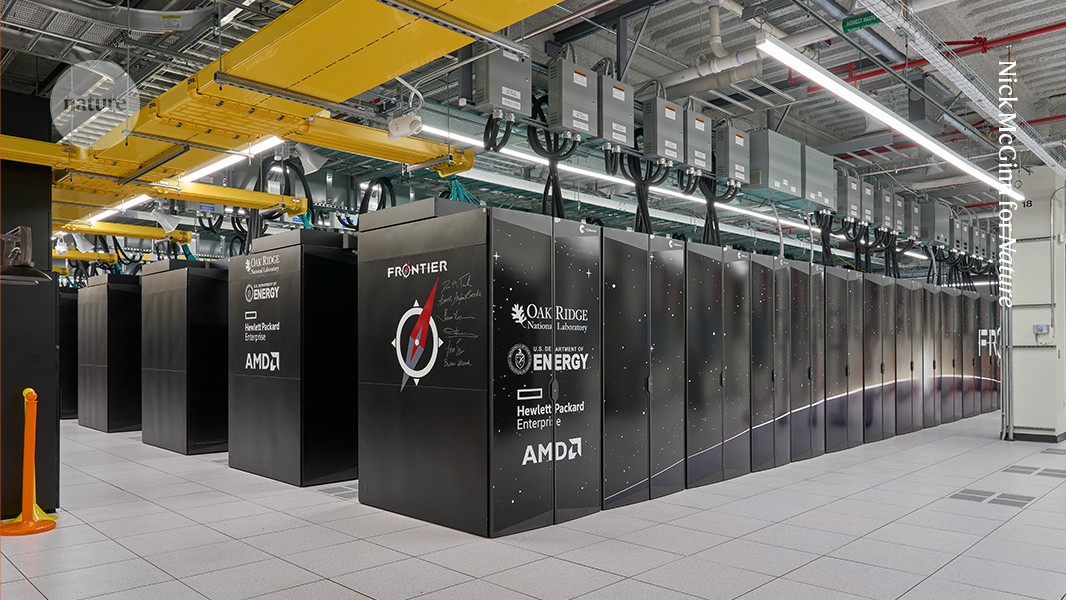
The fastest supercomputer in the world is a machine known as Frontier, but even this speedster with nearly 50,000 processors has its limits. On a sunny Monday in April, its power consumption is spiking as it tries to keep up with the amount of work requested by scientific groups around the world.
The electricity demand peaks at around 27 megawatts, enough to power roughly 10,000 houses, says Bronson Messer, director of science at Oak Ridge National Laboratory in Tennessee, where Frontier is located. With a note of pride in his voice, Messer uses a local term to describe the supercomputer’s work rate: “They are running the machine like a scalded dog.”
Frontier churns through data at record speed, outpacing 100,000 laptops working simultaneously. When it debuted in 2022, it was the first to break through supercomputing’s exascale speed barrier — the capability of executing an exaflop, or 1018 floating point operations per second. The Oak Ridge behemoth is the latest chart-topper in a decades-long global trend of pushing towards larger supercomputers (although it is possible that faster computers exist in military labs or otherwise secret facilities).
How cutting-edge computer chips are speeding up the AI revolution
But speed and size are secondary to Frontier’s main purpose — to push the bounds of human knowledge. Frontier excels at creating simulations that capture large-scale patterns with small-scale details, such as how tiny cloud droplets can affect the pace at which Earth’s climate warms. Researchers are using the supercomputer to create cutting-edge models of everything from subatomic particles to galaxies. Some projects are simulating proteins to help develop new drugs, modelling turbulence to improve aeroplane engine design and creating open-source large language models (LLMs) to compete with the artificial intelligence (AI) tools from Google and OpenAI.
Researchers log on to Frontier from all over the world. In 2023, the supercomputer had 1,744 users in 18 countries. And, in 2024, Oak Ridge anticipates that Frontier users will publish at least 500 papers based on computations performed on the machine.
“Frontier is not unlike the James Webb Space Telescope,” says biophysicist Dilip Asthagiri of Oak Ridge National Laboratory. “We should see it as a scientific instrument.”
Inside the machine
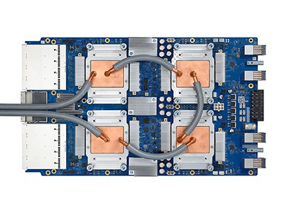
The brains of Frontier reside in a warehouse-sized room filled with a steady electronic hum that is gentle enough to talk over. In the room are 74 identical glossy black racks that hold a total of 9,408 nodes. These are the workhorses of a supercomputer. Each node consists of four graphics processing units (GPUs) and one computer processing unit (CPU).
A team of engineers continuously monitors the machine for signs of trouble, says Corey Edmonds, a technician at Hewlett Packard Enterprise, the company that built the supercomputer. Edmonds, who is based at Oak Ridge, is doing maintenance surgery on Frontier on this day. After fixing a broken connector on one of the nodes, he squeezes grey thermal grease from a syringe on to a silvery rectangle — one of the node’s four GPUs. This helps the GPU to dissipate heat quickly and stay cool.
Frontier owes its speed mainly to its extensive use of GPUs. These chips, first developed to render realistic graphics for computer gamers, are now powering advances in AI through machine-learning applications.
“They can run really fast,” says Messer. “They’re also abysmally stupid.” GPUs excel at crunching many numbers at once — and not much else. “They can do one thing over and over and over and over again,” he says, which makes them useful for speedy work in supercomputer calculations.
Researchers have to customize their code to take advantage of Frontier’s GPUs. Messer likens a scientist using Frontier for the first time to a suburban driver commandeering a race car. “It’s got a steering wheel, gas pedal and a brake,” he says. “But try to get a regular driver into a Formula One car and actually have them go from here to there.”
Big science
It’s not easy for researchers to get a chance to use Frontier. Messer and three colleagues are gathering on this April Monday to evaluate research proposals for the machine. On average, they approve around one in four proposals, and last year awarded time to 131 projects. In particular, applicants need to make the case that their project can take advantage of the supercomputer’s entire system.
The most common allocations they offer are around 500,000 node hours, equivalent to running the entire machine for three days continuously. Their largest allocation is four times bigger. Researchers who are granted time on Frontier get about ten times more computing resources than they can procure anywhere else, says Messer.
Today, his team is doling out smaller awards of around 20,000 node hours, which it does on a weekly basis. Many projects take advantage of Frontier’s ability to simultaneously model a wide range of spatial and time scales. In total, Frontier has about 65 million node-hours available each year.
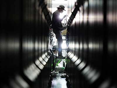
Technicians work on Frontier, which has more than 50,000 processors and is cooled by water.Credit: Nick McGinn for Nature
Scientists want to use Frontier, for example, to simulate atomically accurate biological processes, such as proteins or nucleic acids in solution interacting with other parts of cells.
This May, Asthagiri and Nick Hagerty, a high-performance-computing engineer at Oak Ridge, used Frontier to simulate a cube-shaped drop of liquid water containing more than 155 billion water molecules. “It was to push the machine,” says Asthagiri. The simulated cube is about one-tenth the width of a human hair, and the model is among the largest atomic-level simulations ever made, says Asthagiri, who has not yet published the work in a peer-reviewed journal.
These initial simulations are building towards more ambitious goals to model entire cells from the atoms up. In the near term, researchers would like to simulate a cellular organelle and use these to inform laboratory experiments. They are also working to combine Frontier’s high-resolution simulations of biological materials with ultra-fast imaging using X-ray free-electron lasers to accelerate discoveries.
With Frontier, climate models have become more precise, too. In 2023, Oak Ridge climate scientist Matt Norman and other researchers used the supercomputer to run a global climate model with 3.25-kilometre resolution. Frontier’s computing capability was necessary for them to create a decades-long forecast at this resolution1. The model also incorporated the effects of the complex motion of clouds, which occurs on an even finer resolution. “It took all of Frontier to do it,” says Norman.
Models would run significantly more slowly on other computers to achieve the same resolution while including the effects from clouds, he says. This limitation is a major hurdle for climate scientists seeking to forecast conditions, because cloud behaviour influences the movement of energy around the globe.
Supercomputing poised for a massive speed boost
For a model to be practical for weather and climate forecasts, it needs to run at least one simulated year per day. Frontier could run through 1.26 simulated years per day for this model1, a rate that will allow the researchers to create more-accurate 50-year forecasts than before.
Frontier also brings higher resolution to cosmological scales. Astrophysicist Evan Schneider at the University of Pittsburgh in Pennsylvania is using the supercomputer to study how Milky Way-sized galaxies evolve as they age. Frontier’s galaxy models span four orders of magnitude, up to large-scale galactic structures about 100,000 light years (30,660 parsecs) in size. Before Frontier, the largest structures she could model at comparable resolution were dwarf galaxies, which are about one-fiftieth the mass.
Schneider simulates how supernovae cause gas to leak out of these galaxies2. Over time, thousands to millions of supernova explosions collectively release a significant amount of gas that ultimately exits the galaxy3. Because that gas is the raw material from which new stars are born, star formation slows down as the galaxies age. Frontier allows Schneider to include the effects of hotter gas than is practical with other computers. Her simulations suggest that current cosmological models downplay the role of this hot gas in the evolution of galaxies.
AI researchers are also clamouring for time on Frontier’s GPUs, known for their role in training neural-network-based architectures such as the transformer model underpinning ChatGPT. With its nearly 38,000 GPUs, Frontier occupies a unique public-sector role in the field of AI research, which is otherwise dominated by industry.
Nur Ahmed, an economics researcher now at the University of Arkansas in Fayetteville, and his colleagues highlighted the gap between AI in academia and industry in a commentary last year4. In 2021, 96% of the largest AI models came from industry. On average, industry models were nearly 30 times the size of academic models. The discrepancy is evident in monetary investment, too. Non-defence US agencies provided US$1.5 billion to support AI research in 2021. In that same year, industry spent more than $340 billion globally.
Mind the gap
The gap has only widened since the release of commercial large language models, says Ahmed. The computational resources to train OpenAI’s GPT-4, for example, cost an estimated $78 million, whereas Google spent $191 million to train Gemini Ultra (see go.nature.com/44ihnhx). This gulf in investment leads to a stark asymmetry in the computing resources available to researchers in industry versus academia.
Industry is pushing the boundaries of basic AI research, and this could pose a problem for the field, write Ahmed and his co-authors. Industry dominance could lead to a lack of basic research that is not immediately profitable and result, for example, in the development of AI technologies that neglect the needs of lower-income communities, say the researchers. In an unpublished study, Ahmed has analysed 6 million peer-reviewed articles and 32 million patent citations and found that “on average, industry tends to ignore some of the concerns of marginalized populations in the global south”.
Climate scientists push for access to world’s biggest supercomputers to build better Earth models
What’s more, many models have problems with gender and racial bias, as found in several commercial face-recognition systems based on AI. Academics could serve as auditors to evaluate the risks from AI models, but to do so they need access to computational resources at the same scale as industry, says Ahmed.
That’s where Frontier comes in. Once Oak Ridge approves a project application, the researcher uses the supercomputer for free, as long as they publish their results. That will help university researchers to compete with companies, says computer scientist Abhinav Bhatele at the University of Maryland in College Park. “The only way people in academia can train similar-sized models is if they have access to resources like Frontier,” he says.
Bhatele is using Frontier to develop open-source LLMs as a counterbalance to industry models5. “Often when companies train their models, they keep them proprietary, and they don’t release the model weights,” says Bhatele. “With this open research, we can make these models freely available for anyone to use.” Over the next year, he and his team aim to train a range of LLMs of different sizes, and they will make these models, along with their weights, open-source. They have also made the software for training the models freely available. In this way, says Bhatele, Frontier has a crucial role in a movement in the field to “democratize” AI — to include more people in the technology’s development.
The race continues
A few doors down from the room housing Frontier, its predecessor is still working hard performing jobs for scientists around the world. This machine, called Summit, held the world record for speed between 2018 and 2019 and is currently the world’s ninth-fastest supercomputer among public machines. With its long black chrome racks, Summit resembles Frontier, but has a louder cooling system and works at one-eighth the speed.
Summit’s history hints at Frontier’s future. Frontier first topped the list in 2022, and is likely to surrender that spot before long. The second-place supercomputer, Aurora, based at Argonne National Laboratory in Illinois, is expected to exceed Frontier’s performance at some point with further optimization. Lawrence Livermore National Laboratory’s El Capitan, scheduled to come online later this year at the California-based lab, is also projected to beat Frontier eventually. Also in the mix is Jupiter, an exascale supercomputer in Germany that is due to debut later this year.
Mounting geopolitical tensions further complicate the rankings. Frontier’s title comes from its position on a semiannual ranking from an organization called the TOP500. It rates the world’s supercomputers on the basis of their reported performance on a benchmark task that involves solving a dense set of linear equations.
But computing experts say it is likely that the United States and China are not sharing information publicly about their computing assets, especially because of increasing strain between the two countries. “There is this idea of a kind of a race in supercomputing,” says Kevin Klyman, a policy researcher at the Atlantic Council, a think tank in Washington DC. In fact, in 2022, the administration of US President Joe Biden implemented controls against exporting semiconductors to China, specifically citing concern about China’s supercomputing capability.
In the supercomputing arena, the tensions began years ago. Notably, in 2016, China overtook the United States in the number of supercomputers on the TOP500 list. “That caused a lot of anxiety in the United States,” says Klyman. “A lot of US policymakers said, ‘How do we catch up in the list?’”
Currently, the two countries have the most supercomputers on the TOP500 rankings released this June. The United States boasted 168 machines, whereas China had 80. Researchers wonder, however, whether these countries have powerful supercomputers that they have not disclosed in public. In fact, the number of Chinese machines on the current list has dropped since last November, when it included 104 machines. And China did not report results for any new supercomputers.
Oak Ridge is already planning Frontier’s successor, called Discovery, which should have three to five times the computational speed. It will be the latest in a decades-long quest for speed (see ‘Speed records’). Frontier is 35 times faster than Tianhe-2A, which was the fastest computer in 2014, and 33,000 times faster than Earth Simulator, the fastest supercomputer in 2004.
Researchers are eager for more speed. A bigger computer would allow Schneider, for example, to model galaxies at even higher resolution, she says. It could also give scientists bigger compute budgets.
But engineers face an ongoing challenge: supercomputers consume a lot of energy, and future machines are likely to need even more. So researchers are continuing to push for improvements in energy efficiency. Frontier is more than four times as efficient as Summit, in large part because it is cooled by water at an ambient temperature, unlike Summit, which uses chilled water. About 3–4% of Frontier’s total energy consumption goes to cooling, compared with 10% for Summit.
Energy efficiency has been a key bottleneck for building faster supercomputers for years. “We could have built an exascale supercomputer in 2012, but it just would have been way too expensive to power it,” says Messer. “We would have needed one or two orders of magnitude more power to be able to provide electricity to it.”
As evening settles at the Oak Ridge facility, the hallways on Frontier’s floor are empty save for a skeleton crew. In the supercomputer’s control room, Conner Cunningham is charged with babysitting Frontier for the night. From 7 p.m. to 7 a.m., his job is to make sure no trouble arises as the supercomputer churns through tasks from researchers around the world. He keeps an eye on Frontier using more than a dozen monitors, which display global cybersecurity threats and security-camera footage of the building. A television in the corner shows the local weather on mute, to alert him of any oncoming storms that might interrupt power supplies.
But most nights are quiet enough for Cunningham to study for an online computer science degree from his desk. He’ll perform a few walk-throughs to check for anything unexpected on the premises, but the job is largely passive.
“It’s kind of like with firefighters,” he says. “If anything happens, you need somebody watching.” He’s procured four burritos and some Pepsi to sustain him through his shift. He won’t be sleeping tonight — and neither will Frontier.
United Nations Environment Programme. Zero draft text of the international legally binding instrument on plastic pollution, including in the marine environment. United Nations Environment Assembly of the United Nations Environment Programme. https://wedocs.unep.org/bitstream/handle/20.500.11822/43239/ZERODRAFT.pdf (2023).
Meijer, L. J. J., van Emmerik, T., van der Ent, R., Schmidt, C. & Lebreton, L. More than 1000 rivers account for 80% of global riverine plastic emissions into the ocean. Sci. Adv.7, eaaz5803 (2021).
Ryberg, M. W., Hauschild, M. Z., Wang, F., Averous-Monnery, S. & Laurent, A. Global environmental losses of plastics across their value chains. Resour. Conserv. Recycl.151, 104459 (2019).
MacLeod, M., Domercq, P., Harrison, S. & Praetorius, A. Computational models to confront the complex pollution footprint of plastic in the environment. Nat. Comput. Sci.3, 486–494 (2023).
Zhu, X. & Rochman, C. Emissions inventories of plastic pollution: a critical foundation of an international agreement to inform targets and quantify progress. Environ. Sci. Technol.56, 3309–3312 (2022).
Intergovernmental Panel on Climate Change (IPCC). 2006 IPCC guidelines for national greenhouse gas inventories. Institute for Global Environmental Strategies (IGES) (2006).
Pacyna, E. G., Pacyna, J. M., Steenhuisen, F. & Wilson, S. Global anthropogenic mercury emission inventory for 2000. Atmos. Environ.40, 4048–4063 (2006).
Wilson, S. J., Steenhuisen, F., Pacyna, J. M. & Pacyna, E. G. Mapping the spatial distribution of global anthropogenic mercury atmospheric emission inventories. Atmos. Environ.40, 4621–4632 (2006).
Edelson, M., Håbesland, D. & Traldi, R. Uncertainties in global estimates of plastic waste highlight the need for monitoring frameworks. Mar. Pollut. Bull.171, 112720 (2021).
UN-Habitat. Waste wise cities tool: step by step guide to assess a city’s municipal solid waste management performance through SDG indicator 11.6.1 monitoring. https://unhabitat.org/wwc-tool (2021).
Bank, M. S. et al. Global plastic pollution observation system to aid policy. Environ. Sci. Technol.55, 7770–7775 (2021).
Kantai, T., Hengesbaugh, M., Hovden, K. & Pinto-Bazurco, J. F. Summary of the second meeting of the intergovernmental negotiating committee to develop an international legally binding instrument on plastic pollution: 29 May – 2 June 2023. Earth. Neg. Bull.36, 1–9 (2023).
Fei, X. et al. The distribution, behavior, and release of macro- and micro-size plastic wastes in solid waste disposal sites. Crit. Rev. Environ. Sci. Technol.53, 366–389 (2023).
Velis, C. A. & Cook, E. Mismanagement of plastic waste through open burning with emphasis on the global south: a systematic review of risks to occupational and public health. Environ. Sci. Technol.55, 7186–7207 (2021).
Wiedinmyer, C., Yokelson, R. J. & Gullett, B. K. Global emissions of trace gases, particulate matter, and hazardous air pollutants from open burning of domestic waste. Environ. Sci. Technol.48, 9523–9530 (2014).
Ding, Y. et al. A review of China’s municipal solid waste (MSW) and comparison with international regions: management and technologies in treatment and resource utilization. J. Clean. Prod.293, 126144 (2021).
Chaudhary, P. et al. Underreporting and open burning – the two largest challenges for sustainable waste management in India. Resour. Conserv. Recycl.175, 105865 (2021).
Sharma, G. et al. Gridded emissions of CO, NOx, SO2, CO2, NH3, HCl, CH4, PM2.5, PM10, BC, and NMVOC from open municipal waste burning in India. Environ. Sci. Technol.53, 4765–4774 (2019).
Chen, D. M. C., Bodirsky, B. L., Krueger, T., Mishra, A. & Popp, A. The world’s growing municipal solid waste: trends and impacts. Environ. Res. Lett.15, 074021 (2020).
Schultz, P. W., Bator, R. J., Large, L. B., Bruni, C. M. & Tabanico, J. J. Littering in context: personal and environmental predictors of littering behavior. Environ. Behav.45, 35–59 (2011).
Schiavina, M., Melchiorri, M. & Freire, S. GHS-DUC R2022A – GHS degree of urbanisation classification, application of the degree of urbanisation methodology (stage II) to GADM 3.6 layer, multitemporal (1975-2030). European Commission Joint Research Centre (JRC). http://data.europa.eu/89h/f5224214-6b66-43df-a9c6-cc974f17d803 (2022).
GADM. GADM database of global administrative areas. https://gadm.org/ (2012).
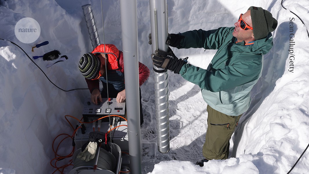
“The sun is shining in this picture, but this isn’t your typical summer’s day — we’re on the summit of the Weißseespitze mountain in Kaunertal, Austria, 3,500 metres above sea level, and it’s −5 °C. My colleagues and I collect ice-core samples from the Gepatschferner glacier, Austria’s second largest, which lies just below the summit. I’m in the green jacket, holding the motor of a mechanical drill to make sure the cutting head is entering the ice at the right angle and speed, while my colleague, glaciologist Martin Stocker-Waldhuber, works the controls.
Fieldwork days start at around 4.30 a.m., because we make four round trips in a helicopter to transport everyone and everything we need to the drilling site. The drill needs a lot of electricity to run, so we have to bring solar panels and batteries with us, as well as all the drill parts.
I’m a technician with the Institute for Interdisciplinary Mountain Research of the Austrian Academy of Sciences in Innsbruck. I often work in temperatures as low as −18 °C, fixing small parts of equipment, so sometimes I can’t wear gloves. It takes a certain type of person to do this: you have to be able to focus when you’re very cold. Everyone on the team is very resilient, knowledgeable and quick to solve problems.
Variations in the layers of the glacier’s ice cores reveal periods of expansion and retreat over 6,000 years. By aligning the history of the glacier with temperature records that have been collected since 1850, we can see how the climate of Europe’s alpine region has changed with global warming and how it’s likely to change in the future. The ice is a climate archive.
I’m in the mountains for around 70 days a year, mostly from May to the end of September. I love this work, because I’m outside using my hands and my brain, and I’m playing a part in achieving a better understanding of our world.”
This interview has been edited for length and clarity.