Tag: multidisciplinary

  • Meet the Latina scientists advancing health and policy

    Meet the Latina scientists advancing health and policy

    [ad_1]

    Life as a scientist in Latin America isn’t always easy — and this is especially true for women. Latina researchers have had to find creative ways to bypass the gender gap from an early age: at 15, girls are half as likely as boys to expect that they’ll work in a science, technology, engineering and mathematics (STEM) area. According to the United Nations, in 2016, less than half (45%) of Latin America’s workforce in research and development were women. Although this figure is above the world average (38%), it is low compared with graduation rates for women in Latin American countries.

    Nature spoke to four Latin American researchers about the peaks and troughs they have faced in their careers and how they are connecting science and policy.

    ILIANA CURIEL: A translator between cultures

    Paediatrician and researcher at the Colombian Institute of Family Welfare in La Guajira, Colombia.

    A portrait of Iliana Curiel

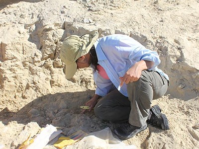
    Iliana Curiel became a paediatrician to help her local community in La Guajira, Colombia.Credit: Iliana Curiel Arismendy

    I am a mix of Black and Wayuu. I grew up in Uribia, a municipality located in La Guajira, Colombia, at the northernmost tip of South America.

    Health challenges in La Guajira are different from those in the rest of Colombia. Although non-transmittable diseases such as obesity and heart conditions demand a considerable effort from public-health services in large cities, the greatest issue in La Guajira is child malnutrition. A child in the region is 60 times more likely to die from undernourishment than is a child living in Bogotá. Most of La Guajira is a desert and access to water can be limited. In some parts of the region, water services reach less than 10% of the population. Around 40% of the population in the territory is under 19, so there is an immense need for paediatric care there. Like other rural and Indigenous communities in Colombia and South America, this is a place where the ‘multidimensional poverty index’ is high and preventable infant and mother mortality abounds.

    Growing up in La Guajira, I decided to be a paediatrician and help my community. But I also wanted more than that: after my medical degree in the mid-1990s, I went on to study public health and social policy.
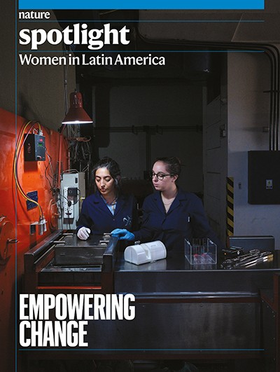
    Indigenous communities in La Guajira do not easily accept Western medicine because their cultural practices differ from those in urban settings — and public-health policies rarely meet on common ground with these cultural singularities. So, in 2018, I went back there and, together with my wife, started a non-governmental organization, Los Hijos del Sol (Children of the Sun). Our goal has been to conduct research by listening to Indigenous communities, allowing us to plan more adequate models of health care.

    Once, for example, we needed to care for a severely undernourished boy. But to offer proper care, we needed to take him from the community to a hospital — and to do that, we had to ask for permission from the community leaders. Because we were in a matrilineal-led group — in which the line of descent is considered from the mothers’ side — it was the boy’s maternal uncles, not his parents, who spoke for the child. So we had to contact his uncle first. A health team, unaware of this, might have asked the boy’s mother for authorization and had a hard time gaining it. If the family think a certain disease is rooted in a spell or bad spirits, we can’t say it’s nonsense — we must adapt our approach and find a shared understanding.

    At Los Hijos del Sol, we train Indigenous mothers and midwives to take steps to reduce child mortality. We ask mothers how they know when their child is in trouble, and they come up with the most beautiful analogies. They won’t say the child is “breathing quickly”, but that the child is in a “high tide”, as if the chest and abdomen were moving like restless waves — and they know that it is a sign of alarm.

    Most physicians avoid politics, but public health is a political matter and we must be aware of that if we ever want to change things for the better. I’d tell young Latina researchers to never lose sight of your purpose. The path in science, to women, is one of perseverance and resistance, but also of transformation. The qualities that are said to disqualify us as scientists — such as empathy and creativity — are the ones we should take most pride in.

    Iliana Curiel providing care to a newborn baby

    Child malnutrition in La Guajira is one of the biggest issues in the region, says Iliana Curiel (left).Credit: Organización Los Hijos del Sol

    XÓCHITL CASTAÑEDA: A voice to Latin American immigrants

    Programme director and professor in the School of Public Health at the University of California, Berkeley.

    Around 30 years ago, I moved from Mexico City to the United States for my postdoctoral research and it was here that I first saw the negative health impacts felt by immigrants. In the early 2000s, a large number of the migrant community came from Mexico and Latin America. Although the number of migrants from other countries has grown, Mexicans are still the main immigrant workforce in the United States — we’re about 10.6 million people.

    During my research at the University of California in San Francisco, I visited the fields where farm workers were employed, and it completely changed my life. I saw the terrible conditions in which they were living to perform the most dangerous, belittling and dirty jobs.

    I am a medical anthropologist; in the mid-1990s, I was conducting research on the risks that immigrants faced regarding HIV and AIDS. After witnessing neglect and abuse of migrant workers, I realized I couldn’t just stay in academia — I needed to translate research into public action. And this was the beginning of the Health Initiative of the Americas, a programme on health and migration at the University of California, Berkeley.

    Since its inception in 2001, the programme has relied on around 20,000 volunteers working to grow a grass-roots movement. I was very fortunate to be part of the University of California system: it helped me to knock at the door of the Mexican government. Because of the magnitude of the Mexican diaspora in the United States, the Mexican government has 50 consulates in the United States. The Mexican government partnered with the programme, and this has opened the doors to cooperation with other Latin American countries, such as Guatemala, El Salvador and Honduras. In the United States, health is unfortunately not a human right — it is sometimes seen as a commodity. We want to extend access to health care to immigrants, who are excluded from the health system, to help improve their living conditions.

    We wanted to hold National Health Weeks, just like the ones in Mexico — when the government mobilizes health personnel across the country to knock at houses to give everyone a chance to get vaccinated three times a year. But without accredited health providers, that wouldn’t be possible in the United States. So, we sought out community clinics, and many other organizations started to join: our network has several partners nationwide, including health and cultural institutions and consulates. These are places where immigrants, regardless of their legal status, can access basic health services and advice. Even in remote regions of the United States, they can get vaccines and education about preventive health to improve their overall quality of life.

    Young Latina researchers have the opportunity and the responsibility to contribute to a more equitable world. My advice is to never give up. Even in hard times there is light, and public health is a marvellous instrument to shine that light.

    DENISE LAPA: A fetoscopy pioneer

    Fetal and neonatal surgery programme coordinator at Sabará Child Hospital in São Paulo, Brazil.

    In 1999, I started to develop a technique to treat spina bifida — a pre-birth condition in which the neural tube bulges on the back of the fetus. The condition can damage nerves in the spinal cord and greatly affect a child’s ability to walk or perform day-to-day activities.

    In the late 1990s, Thomas Kohl, who is now head of the German Center for Fetal Surgery and Minimally-Invasive Therapy at the University Medical Center Mannheim, developed a technique to close the gap that forms in the spine. His idea was to stitch the fetus’s spine without opening the mother’s womb. I had been testing a similar technique for a decade when, in 2012, he invited me to Germany. We started an informal exchange.

    The difference between Kohl’s technique and mine was that, instead of stitching all of the layers in the back of a fetus — spinal cord, muscle and skin tissues — my team and I used a biocellulose patch over the spinal tissue to help it self-heal and avoid suturing the fetus’s spinal cord to the tissue above it.

    Throughout my career, I felt I had to prove myself all the time as a woman and, as a Latina researcher, I also had regional prejudice on top of that. To me, it seemed that some people, most of whom were men, felt that if a breakthrough in fetoscopy (fetal endoscopy) was to be made, it wouldn’t be made by a woman and certainly not one from Brazil.

    However, in 2013, after 14 years of testing in animal models, our first fetal surgery at the Samaritan Hospital of São Paulo proved that the technique worked. A decade later, we could see that not only was it viable, but also that it yielded positive long-term results. A study1 following 78 children who had undergone our procedure showed that almost half of them (46%) could walk independently once they reached between 2.5 and 10 years old — and almost all of them (94%) had expected social function. In comparison, a 2020 study2 on the effectiveness of the conventional open-womb surgical technique showed that around 29% of children aged 6 and over who had undergone this surgery could walk independently. Previous studies have shown that the effectiveness of the conventional technique in terms of walking rates is as high as 45%3.

    As well as in Brazil, our technique is now used in Israel, Chile, Uruguay, Italy and parts of the United States. It’s also rising in popularity: more than 300 surgeries have been performed outside Brazil. Everything I did in my life, I accomplished because a man told me I couldn’t. It’s extremely rewarding to see children, whose parents relied on my team, being able not only to walk, but also to jump and play freely — some even go skiing and do ballet.

    My piece of advice to young Latina researchers would be: structural sexism is still not understood by most men. It is up to us, women, to occupy important spaces and teach our daughters a different language of love and respect between men and women.

    YESTER BASMADJIÁN:On the front line against insect-borne diseases

    Head of the Department of Parasitology and Mycology in the Medicine Faculty at the University of the Republic in Montevideo, Uruguay.

    Yester Basmadjián sitting at her desk

    Yester Basmadjián says protecting against misinformation is an important part of her job.Credit: Ramiro Tomasina

    Before the viral disease dengue returned to Uruguay in 2016, the last epidemic had been a century earlier, in 1916. In the late 1950s, the country had eradicated the mosquito vector Aedes aegypti through monitoring populations and their behaviour. But, because the continent never fully got rid of it, the mosquito returned in 1997. Despite heavy public campaigning, the country was unable to eradicate it again. Now we’re seeing a rise in local transmission of dengue, especially in the Montevideo region and Salto on the border with Argentina. There were 48 confirmed cases in 2023, and this year we have seen more than 700.

    Cases of dengue, most of which were imported by travellers from neighbouring countries such as Brazil, Argentina and Paraguay, are now a concern in Montevideo. At the University of the Republic in Montevideo, we have a laboratory in which we can study this and other disease-vector insects more closely. Our lab has the support of Uruguay’s Public Health Ministry, the International Atomic Energy Agency (IAEA) and the Pan American Health Organization, and we have partnered with a number of institutions in Brazil and other Latin American countries.

    We’re using X-rays (hence our partnership with the IAEA) to sterilize male A. aegypti mosquitoes before they become adults, to decrease their overall population. Female mosquitoes mate only once; if they mate with sterile males then they won’t produce offspring. Another advantage is that male mosquitoes generally don’t interact with people and, because they do not feed on blood, they don’t transmit diseases. Our project will not eliminate this insect in Uruguay, but it’s a tool that will add to the fight. It is certainly better than open-air insecticide spraying — we don’t know whether mosquitoes in Uruguay are resistant to certain chemicals. We’re launching close to 30,000 first-generation sterile mosquitoes at the end of this year and are looking forward to good results.

    One of our biggest challenges is ensuring that the new lab remains operational in both the medium and long term — not only by maintaining resources, but also by protecting against a wave of misinformation and conspiracy theories. Many people think that sterilization of mosquitoes is going to cause a change in human bodies (which is not possible even if a male mosquito interacted with a person). At the lab, we try to counter this through outreach with journalists and by promoting workshops in schools.

    Although sterilizing mosquitoes is not a silver bullet to end dengue, it’s an important tool, and the public’s cooperation is essential to fight the mosquito that transmits it.

    My advice to young Latina researchers is that we have to study a lot to adapt to an ever more technological world — but it’s important never to give up when faced with challenges. Always move forward and, at some point, you’ll get to where you want to be.

    [ad_2]

    Source link

  • Constraint reveals the mitochondrial genome sites most important for health and disease

    Constraint reveals the mitochondrial genome sites most important for health and disease

    [ad_1]

    • RESEARCH BRIEFINGS

    Mitochondrial DNA (mtDNA) is the part of the genome found in mitochondria, the ‘powerhouses’ of the cell. An analysis of mitochondrial genomes from nearly 60,000 people shows where selection has removed deleterious genetic variants from the population, revealing which mtDNA sites are most important for human health and disease.

    [ad_2]

    Source link

  • Gingras, A. C., Raught, B. & Sonenberg, N. eIF4 initiation factors: effectors of mRNA recruitment to ribosomes and regulators of translation. Annu. Rev. Biochem. 68, 913–963 (1999).

    Article 
    CAS 
    PubMed 

    Google Scholar
     

  • Hinnebusch, A. G. & Lorsch, J. R. The mechanism of eukaryotic translation initiation: new insights and challenges. Cold Spring Harb. Perspect. Biol. 4, a011544 (2012).

    Article 
    PubMed 
    PubMed Central 

    Google Scholar
     

  • Merrick, W. C. eIF4F: a retrospective. J. Biol. Chem. 290, 24091–24099 (2015).

    Article 
    CAS 
    PubMed 
    PubMed Central 

    Google Scholar
     

  • Abramson, R. D. et al. The ATP-dependent interaction of eukaryotic initiation factors with mRNA. J. Biol. Chem. 262, 3826–3832 (1987).

    Article 
    CAS 
    PubMed 

    Google Scholar
     

  • Kaye, N. M., Emmett, K. J., Merrick, W. C. & Jankowsky, E. Intrinsic RNA binding by the eukaryotic initiation factor 4F depends on a minimal RNA length but not on the m7G cap. J. Biol. Chem. 284, 17742–17750 (2009).

    Article 
    CAS 
    PubMed 
    PubMed Central 

    Google Scholar
     

  • von der Haar, T. & McCarthy, J. E. Intracellular translation initiation factor levels in Saccharomyces cerevisiae and their role in cap-complex function. Mol. Microbiol. 46, 531–544 (2002).

    Article 
    PubMed 

    Google Scholar
     

  • Martinez-Salas, E., Francisco-Velilla, R., Fernandez-Chamorro, J. & Embarek, A. M. Insights into structural and mechanistic features of viral IRES elements. Front. Microbiol. 8, 2629 (2017).

    Article 
    PubMed 

    Google Scholar
     

  • Jia, Y., Polunovsky, V., Bitterman, P. B. & Wagner, C. R. Cap-dependent translation initiation factor eIF4E: an emerging anticancer drug target. Med. Res. Rev. 32, 786–814 (2012).

    Article 
    CAS 
    PubMed 
    PubMed Central 

    Google Scholar
     

  • Otero, L. J., Ashe, M. P. & Sachs, A. B. The yeast poly(A)-binding protein Pab1p stimulates in vitro poly(A)-dependent and cap-dependent translation by distinct mechanisms. EMBO J. 18, 3153–3163 (1999).

    Article 
    CAS 
    PubMed 
    PubMed Central 

    Google Scholar
     

  • He, H. et al. The yeast eukaryotic initiation factor 4G (eIF4G) HEAT domain interacts with eIF1 and eIF5 and is involved in stringent AUG selection. Mol. Cell. Biol. 23, 5431–5445 (2003).

    Article 
    CAS 
    PubMed 
    PubMed Central 

    Google Scholar
     

  • Yourik, P. et al. Yeast eIF4A enhances recruitment of mRNAs regardless of their structural complexity. eLife 6, e31476 (2017).

    Article 
    PubMed 
    PubMed Central 

    Google Scholar
     

  • Kumar, P., Hellen, C. U. & Pestova, T. V. Toward the mechanism of eIF4F-mediated ribosomal attachment to mammalian capped mRNAs. Genes Dev. 30, 1573–1588 (2016).

    Article 
    CAS 
    PubMed 
    PubMed Central 

    Google Scholar
     

  • Gruner, S. et al. The structures of eIF4E-eIF4G complexes reveal an extended interface to regulate translation initiation. Mol. Cell 64, 467–479 (2016).

    Article 
    PubMed 

    Google Scholar
     

  • Oberer, M., Marintchev, A. & Wagner, G. Structural basis for the enhancement of eIF4A helicase activity by eIF4G. Genes Dev. 19, 2212–2223 (2005).

    Article 
    CAS 
    PubMed 
    PubMed Central 

    Google Scholar
     

  • Rajagopal, V., Park, E. H., Hinnebusch, A. G. & Lorsch, J. R. Specific domains in yeast translation initiation factor eIF4G strongly bias RNA unwinding activity of the eIF4F complex toward duplexes with 5′-overhangs. J. Biol. Chem. 287, 20301–20312 (2012).

    Article 
    CAS 
    PubMed 
    PubMed Central 

    Google Scholar
     

  • Cetin, B. & O’Leary, S. E. mRNA- and factor-driven dynamic variability controls eIF4F-cap recognition for translation initiation. Nucleic Acids Res. 50, 8240–8261 (2022).

    Article 
    CAS 
    PubMed 
    PubMed Central 

    Google Scholar
     

  • O’Sullivan, M. H. & Fraser, C. S. Monitoring RNA restructuring in a human cell-free extract reveals eIF4A-dependent and eIF4A-independent unwinding activity. J. Biol. Chem. 299, 104936 (2023).

    Article 
    PubMed 
    PubMed Central 

    Google Scholar
     

  • Lanker, S. et al. Interactions of the eIF-4F subunits in the yeast Saccharomyces cerevisiae. J. Biol. Chem. 267, 21167–21171 (1992).

    Article 
    CAS 
    PubMed 

    Google Scholar
     

  • Feoktistova, K., Tuvshintogs, E., Do, A. & Fraser, C. S. Human eIF4E promotes mRNA restructuring by stimulating eIF4A helicase activity. Proc. Natl Acad. Sci. USA 110, 13339–13344 (2013).

    Article 
    ADS 
    CAS 
    PubMed 
    PubMed Central 

    Google Scholar
     

  • Cetin, B., Song, G. J. & O’Leary, S. E. Heterogeneous dynamics of protein-RNA interactions across transcriptome-derived messenger RNA populations. J. Am. Chem. Soc. 142, 21249–21253 (2020).

    Article 
    CAS 
    PubMed 
    PubMed Central 

    Google Scholar
     

  • Sokabe, M. & Fraser, C. S. A helicase-independent activity of eIF4A in promoting mRNA recruitment to the human ribosome. Proc. Natl Acad. Sci. USA 114, 6304–6309 (2017).

    Article 
    ADS 
    CAS 
    PubMed 
    PubMed Central 

    Google Scholar
     

  • Sen, N. D., Zhou, F., Ingolia, N. T. & Hinnebusch, A. G. Genome-wide analysis of translational efficiency reveals distinct but overlapping functions of yeast DEAD-box RNA helicases Ded1 and eIF4A. Genome Res. 25, 1196–1205 (2015).

    Article 
    CAS 
    PubMed 
    PubMed Central 

    Google Scholar
     

  • Harms, U., Andreou, A. Z., Gubaev, A. & Klostermeier, D. eIF4B, eIF4G and RNA regulate eIF4A activity in translation initiation by modulating the eIF4A conformational cycle. Nucleic Acids Res. 42, 7911–7922 (2014).

    Article 
    CAS 
    PubMed 
    PubMed Central 

    Google Scholar
     

  • Andreou, A. Z. & Klostermeier, D. eIF4B and eIF4G jointly stimulate eIF4A ATPase and unwinding activities by modulation of the eIF4A conformational cycle. J. Mol. Biol. 426, 51–61 (2014).

    Article 
    CAS 
    PubMed 

    Google Scholar
     

  • O’Leary, S. E., Petrov, A., Chen, J. & Puglisi, J. D. Dynamic recognition of the mRNA cap by Saccharomyces cerevisiae eIF4E. Structure 21, 2197–2207 (2013).

    Article 
    PubMed 

    Google Scholar
     

  • Krause, L., Willing, F., Andreou, A. Z. & Klostermeier, D. The domains of yeast eIF4G, eIF4E and the cap fine-tune eIF4A activities through an intricate network of stimulatory and inhibitory effects. Nucleic Acids Res. 50, 6497–6510 (2022).

    Article 
    CAS 
    PubMed 
    PubMed Central 

    Google Scholar
     

  • Schutz, P. et al. Crystal structure of the yeast eIF4A-eIF4G complex: an RNA-helicase controlled by protein-protein interactions. Proc. Natl Acad. Sci. USA 105, 9564–9569 (2008).

    Article 
    ADS 
    CAS 
    PubMed 
    PubMed Central 

    Google Scholar
     

  • Rozen, F. et al. Bidirectional RNA helicase activity of eucaryotic translation initiation factors 4A and 4F. Mol. Cell. Biol. 10, 1134–1144 (1990).

    CAS 
    PubMed 
    PubMed Central 

    Google Scholar
     

  • Ray, B. K. et al. ATP-dependent unwinding of messenger RNA structure by eukaryotic initiation factors. J. Biol. Chem. 260, 7651–7658 (1985).

    Article 
    CAS 
    PubMed 

    Google Scholar
     

  • Mitchell, S. F. et al. The 5′-7-methylguanosine cap on eukaryotic mRNAs serves both to stimulate canonical translation initiation and to block an alternative pathway. Mol. Cell 39, 950–962 (2010).

    Article 
    CAS 
    PubMed 
    PubMed Central 

    Google Scholar
     

  • Marcotrigiano, J. et al. A conserved HEAT domain within eIF4G directs assembly of the translation initiation machinery. Mol. Cell 7, 193–203 (2001).

    Article 
    CAS 
    PubMed 

    Google Scholar
     

  • Hershey, P. E. et al. The Cap-binding protein eIF4E promotes folding of a functional domain of yeast translation initiation factor eIF4G1. J. Biol. Chem. 274, 21297–21304 (1999).

    Article 
    CAS 
    PubMed 

    Google Scholar
     

  • Rogers, G. W. Jr, Komar, A. A. & Merrick, W. C. eIF4A: the godfather of the DEAD box helicases. Prog. Nucleic Acid Res. Mol. Biol. 72, 307–331 (2002).

    Article 
    CAS 
    PubMed 

    Google Scholar
     

  • Lindqvist, L., Imataka, H. & Pelletier, J. Cap-dependent eukaryotic initiation factor-mRNA interactions probed by cross-linking. RNA 14, 960–969 (2008).

    Article 
    CAS 
    PubMed 
    PubMed Central 

    Google Scholar
     

  • Liu, X., Schuessler, P. J., Sahoo, A. & Walker, S. E. Reconstitution and analyses of RNA interactions with eukaryotic translation initiation factors and ribosomal preinitiation complexes. Methods 162-163, 42–53 (2019).

    Article 
    CAS 
    PubMed 
    PubMed Central 

    Google Scholar
     

  • Hilbert, M., Kebbel, F., Gubaev, A. & Klostermeier, D. eIF4G stimulates the activity of the DEAD box protein eIF4A by a conformational guidance mechanism. Nucleic Acids Res. 39, 2260–2270 (2011).

    Article 
    CAS 
    PubMed 

    Google Scholar
     

  • Andreou, A. Z., Harms, U. & Klostermeier, D. eIF4B stimulates eIF4A ATPase and unwinding activities by direct interaction through its 7-repeats region. RNA Biol. 14, 113–123 (2017).

    Article 
    PubMed 

    Google Scholar
     

  • Querido, J. B. et al. The structure of a human translation initiation complex reveals two independent roles for the helicase eIF4A. Nat. Struct. Mol. Biol. 31, 455–464 (2024).

  • Haizel, S. A., Bhardwaj, U., Gonzalez, R. L. Jr, Mitra, S. & Goss, D. J. 5′-UTR recruitment of the translation initiation factor eIF4GI or DAP5 drives cap-independent translation of a subset of human mRNAs. J. Biol. Chem. 295, 11693–11706 (2020).

    Article 
    CAS 
    PubMed 
    PubMed Central 

    Google Scholar
     

  • Acker, M. G., Kolitz, S. E., Mitchell, S. F., Nanda, J. S. & Lorsch, J. R. Reconstitution of yeast translation initiation. Methods Enzymol. 430, 111–145 (2007).

    Article 
    CAS 
    PubMed 

    Google Scholar
     

  • Wang, J. et al. eIF5B gates the transition from translation initiation to elongation. Nature 573, 605–608 (2019).

    Article 
    ADS 
    CAS 
    PubMed 
    PubMed Central 

    Google Scholar
     

  • Jarmoskaite, I., AlSadhan, I., Vaidyanathan, P. P. & Herschlag, D. How to measure and evaluate binding affinities. eLife 9, e57264 (2020).

    Article 
    CAS 
    PubMed 
    PubMed Central 

    Google Scholar
     

  • Buttner, L., Javadi-Zarnaghi, F. & Hobartner, C. Site-specific labeling of RNA at internal ribose hydroxyl groups: terbium-assisted deoxyribozymes at work. J. Am. Chem. Soc. 136, 8131–8137 (2014).

    Article 
    PubMed 

    Google Scholar
     

  • Graham, J. S., Johnson, R. C. & Marko, J. F. Concentration-dependent exchange accelerates turnover of proteins bound to double-stranded DNA. Nucleic Acids Res. 39, 2249–2259 (2011).

    Article 
    CAS 
    PubMed 

    Google Scholar
     

  • Kamar, R. I. et al. Facilitated dissociation of transcription factors from single DNA binding sites. Proc. Natl Acad. Sci. USA 114, E3251–E3257 (2017).

    Article 
    CAS 
    PubMed 
    PubMed Central 

    Google Scholar
     

  • Kosar, Z., Attar, A. G. & Erbas, A. Facilitated dissociation of nucleoid-associated proteins from DNA in the bacterial confinement. Biophys. J. 121, 1119–1133 (2022).

    Article 
    ADS 
    CAS 
    PubMed 
    PubMed Central 

    Google Scholar
     

  • Luo, Y., North, J. A., Rose, S. D. & Poirier, M. G. Nucleosomes accelerate transcription factor dissociation. Nucleic Acids Res. 42, 3017–3027 (2014).

    Article 
    CAS 
    PubMed 

    Google Scholar
     

  • MacDougall, D. D. & Gonzalez, R. L. Jr Translation initiation factor 3 regulates switching between different modes of ribosomal subunit joining. J. Mol. Biol. 427, 1801–1818 (2015).

    Article 
    CAS 
    PubMed 

    Google Scholar
     

  • Wang, J. et al. Rapid 40S scanning and its regulation by mRNA structure during eukaryotic translation initiation. Cell 185, 4474–4487 (2022).

    Article 
    CAS 
    PubMed 
    PubMed Central 

    Google Scholar
     

  • Rajyaguru, P., She, M. & Parker, R. Scd6 targets eIF4G to repress translation: RGG motif proteins as a class of eIF4G-binding proteins. Mol. Cell 45, 244–254 (2012).

    Article 
    CAS 
    PubMed 
    PubMed Central 

    Google Scholar
     

  • Gupta, N., Lorsch, J. R. & Hinnebusch, A. G. Yeast Ded1 promotes 48S translation pre-initiation complex assembly in an mRNA-specific and eIF4F-dependent manner. eLife 7, e38892 (2018).

    Article 
    PubMed 
    PubMed Central 

    Google Scholar
     

  • Linder, P. & Jankowsky, E. From unwinding to clamping—the DEAD box RNA helicase family. Nat. Rev. Mol. Cell Biol. 12, 505–516 (2011).

    Article 
    CAS 
    PubMed 

    Google Scholar
     

  • Sen, N. D. et al. Functional interplay between DEAD-box RNA helicases Ded1 and Dbp1 in preinitiation complex attachment and scanning on structured mRNAs in vivo. Nucleic Acids Res. 47, 8785–8806 (2019).

    CAS 
    PubMed 
    PubMed Central 

    Google Scholar
     

  • Sharma, D. & Jankowsky, E. The Ded1/DDX3 subfamily of DEAD-box RNA helicases. Crit. Rev. Biochem. Mol. Biol. 49, 343–360 (2014).

    Article 
    CAS 
    PubMed 

    Google Scholar
     

  • Brito Querido, J. et al. The structure of a human translation initiation complex reveals two independent roles for the helicase eIF4A. Nat. Struct. Mol. Biol. 31, 455–464 (2024).

    Article 
    CAS 
    PubMed 
    PubMed Central 

    Google Scholar
     

  • Bohlen, J., Fenzl, K., Kramer, G., Bukau, B. & Teleman, A. A. Selective 40S footprinting reveals cap-tethered ribosome scanning in human cells. Mol. Cell 79, 561–574 (2020).

    Article 
    CAS 
    PubMed 

    Google Scholar
     

  • Pause, A., Methot, N., Svitkin, Y., Merrick, W. C. & Sonenberg, N. Dominant negative mutants of mammalian translation initiation factor eIF-4A define a critical role for eIF-4F in cap-dependent and cap-independent initiation of translation. EMBO J. 13, 1205–1215 (1994).

    Article 
    CAS 
    PubMed 
    PubMed Central 

    Google Scholar
     

  • Livingston, N. M. et al. Bursting translation on single mRNAs in live cells. Mol. Cell 83, 2276–2289 (2023).

    Article 
    CAS 
    PubMed 
    PubMed Central 

    Google Scholar
     

  • Zinshteyn, B., Rojas-Duran, M. F. & Gilbert, W. V. Translation initiation factor eIF4G1 preferentially binds yeast transcript leaders containing conserved oligo-uridine motifs. RNA 23, 1365–1375 (2017).

    Article 
    CAS 
    PubMed 
    PubMed Central 

    Google Scholar
     

  • Tamarkin-Ben-Harush, A., Vasseur, J. J., Debart, F., Ulitsky, I. & Dikstein, R. Cap-proximal nucleotides via differential eIF4E binding and alternative promoter usage mediate translational response to energy stress. eLife 6, e21907 (2017).

    Article 
    PubMed 
    PubMed Central 

    Google Scholar
     

  • Lakowicz, J. R. Principles of Fluorescence Spectroscopy 3rd edn (Springer, 2006).

  • Blanchard, S. C., Kim, H. D., Gonzalez, R. L. Jr, Puglisi, J. D. & Chu, S. tRNA dynamics on the ribosome during translation. Proc. Natl Acad. Sci. USA 101, 12893–12898 (2004).

    Article 
    ADS 
    CAS 
    PubMed 
    PubMed Central 

    Google Scholar
     

  • Blanchard, S. C., Gonzalez, R. L., Kim, H. D., Chu, S. & Puglisi, J. D. tRNA selection and kinetic proofreading in translation. Nat. Struct. Mol. Biol. 11, 1008–1014 (2004).

    Article 
    CAS 
    PubMed 

    Google Scholar
     

  • Edelstein, A., Amodaj, N., Hoover, K., Vale, R. & Stuurman, N. Computer control of microscopes using microManager. Curr. Protoc. Mol. Biol. https://doi.org/10.1002/0471142727.mb1420s92 (2010).

  • Ray, K. K. et al. Entropic control of the free-energy landscape of an archetypal biomolecular machine. Proc. Natl Acad. Sci. USA 120, e2220591120 (2023).

    Article 
    CAS 
    PubMed 
    PubMed Central 

    Google Scholar
     

  • Verma, A. R. et al. Increasing the accuracy of single-molecule data analysis using tMAVEN. Biophys J. 123, 2765–2780 (2024).

  • Bronson, J. E., Fei, J., Hofman, J. M., Gonzalez, R. L. Jr & Wiggins, C. H. Learning rates and states from biophysical time series: a Bayesian approach to model selection and single-molecule FRET data. Biophys. J. 97, 3196–3205 (2009).

    Article 
    ADS 
    CAS 
    PubMed 
    PubMed Central 

    Google Scholar
     

  • Schindelin, J. et al. Fiji: an open-source platform for biological-image analysis. Nat. Methods 9, 676–682 (2012).

    Article 
    CAS 
    PubMed 

    Google Scholar
     

[ad_2]

Source link

  • Why Asia is leading the field in green materials

    Why Asia is leading the field in green materials

    [ad_1]

    A man in a hard hat and overalls looks at large rollers of thin silver materials overhead

    A worker checks on the production of low-carbon materials in Huaibei, eastern China.Credit: NurPhoto/Getty

    Buying an ice cream in hot weather presents a challenge for those who prefer to linger over their summer snack: it can be a matter of seconds before even the hardiest product turns to soup. An experiment by a team of researchers in China provides some hope for those with such time-management issues. Their biodegradable ‘passive cooling’ wrapper — which works, in part, by radiating heat into space — kept an ice cream perfectly intact for 80 minutes after being placed in the sunshine1.

    The experiment had an important motive. According to Jia Zhu, a materials-science researcher at Nanjing University who led the work, it showed that such materials have huge potential in a warming climate. When an 80 m2 sheet of the same material was laid on the surface of China’s Tianshan Glacier No. 1 in Xinjiang, the covered section was about 70 cm higher after 20 days. Other researchers have used similar materials on rooftops to cool buildings without consuming energy.

    The hunt for passive-cooling solutions is one example of the surge in materials-based green-technology research under way across Asia, a focus that might be a factor behind Asian countries’ increasing dominance in materials science in the Nature Index. In 2023, China, Japan, South Korea, India and Singapore all made the global top 10 for materials-science output by country. Together, their combined Share (the metric that measures a country or institution’s output in Index journals) accounted for 63% of global output in the field.

    Much of the green-materials work is dominated by research on next-generation batteries and solar cells, but numerous other technologies are under investigation, often with a focus on materials designed to interact with sunlight in unusual and potentially useful ways.

    “In nature, light and heat are the two most powerful forms of energy,” Zhu says. “I explore ways to manipulate light and heat using hierarchically structured materials.” The ice-cream study showed hierarchical structure in action. At the microscale, pores in the plant-derived cellulose acetate film scatter and reflect incoming sunlight, bouncing solar heat away. At the nanoscale, the film’s atomic structure radiates heat within a band of infrared light known as the atmospheric transparent window. This heat is not reabsorbed by any atmospheric gases and is lost to space — using the Universe as a vast heat sink to keep objects on Earth cool.

    By keeping objects cool without consuming energy, such radiative cooling materials could be key to combating rising urban heat, says materials scientist Xiaobo Yin, who develops passive-cooling materials at the University of Hong Kong. “Air conditioning moves heat from inside the house to the outside, while consuming energy which adds more heat to the environment,” Yin says. “Buildings or roads capable of radiative cooling are the only way we can expel the excess heat out of the Earth.”

    Asia’s mega-cities are among the places where passive cooling will be most important, says Yin, who moved to Hong Kong from the United States in 2021. It is one reason why research into sustainable materials is a priority in many Asian countries. According to Zhu, it also helps that there is a consensus on the need for action to deal with climate change. “I don’t think people in China have any doubt that climate change is real,” he says.

    Zhu, who spent almost a decade studying and working in the United States — at Stanford University in California and the University of California, Berkeley — before joining Nanjing University in 2013, also points to the existing evidence that environmental challenges can be met through technology. When he returned to China, for instance, atmospheric pollution in cities was rife. “It was very clear how industrialization was impacting the wider environment,” he says. But a range of government measures — including encouraging electric-vehicle uptake — have since made a difference, he says.

    Bin Liu pictured in a lab next to a setup with glass tubes containing coloured liquid substances behind safety glass

    Bin Liu, director of the National University of Singapore’s Flagship Green Energy Programme.Credit: National University of Singapore

    Green-energy materials research is also important for the economy of many East Asian countries, Zhu adds, given their “heavy emphasis on manufacturing”, an energy-intensive process that could be made cheaper and less carbon-intensive by transitioning to renewable energy. There is also great potential to export novel green-energy technologies.

    “Materials-science research is well supported in countries like India and China because they have recognized the potential for fundamental research to promote their manufacturing industry,” says Tianyi Ma, a materials scientist at RMIT University in Melbourne, Australia.

    Asian countries also typically do very well in terms of investing funding into the translational phase of research to better connect academic ideas with industry, Ma adds. “It’s a win–win situation because in return, industry partners offer more financial support for fundamental research.”

    Rose-tinted research

    Aside from materials that reject sunlight to provide cooling, another highly active area of research in Asia is to develop materials that capture and use sunlight for sustainability gains. Yin’s latest focus was to develop a semi-translucent material that captures green light from the Sun and re-emits it as red light. “We’re trying to tailor the solar spectrum for better crops,” Yin says. Plants rarely use the green light in sunlight for photosynthesis — hence, leaves appear green as this light is reflected — so turning the green part of the solar spectrum into red light converts it into a form that plants can use.

    Proportion bar chart showing how Nature Index research output is split between the leading ten countries in the world

    Source: Nature Index

    By tuning the solar spectrum in this way2, the microphotonic film, which Yin first worked on with colleagues while in the United States, boosted the growth of lettuces by more than 20%. The same gains were seen for plants grown under lights. “For vertical farming or vegetable factories, the primary energy cost is lighting,” Yin says. “It’s an area where our work could contribute.”

    The team is developing a version of the film for sustainable biomanufacturing3. “We also want to tailor the solar spectrum for the fast growth of microalgae,” Yin says. The idea is to use microalgae to turn carbon dioxide emissions into valuable products, because the microalgae absorb CO2 as they grow, becoming rich in proteins and oils that can be harvested. The team is first targeting niche, high-value superfood or cosmetics applications. “But the more we scale up, the lower production costs, and the broader the range of products we could consider,” Yin says.

    Harnessing light to drive the conversion of CO2 into valuable products is also a hot topic in Singapore, where the government prioritizes sustainable-materials research, although for different reasons than the region’s major manufacturing economies.

    “Singapore is very short of natural resources,” says Bin Liu, a materials-science researcher at the National University of Singapore, and director of the university’s Flagship Green Energy Programme. “If we can convert CO2 emissions into a large-scale green fuel, that will solve sustainability and also energy-import issues in Singapore,” she says. “The government’s five-year plan has prioritized this area, so the funding support is tremendous in materials.”

    Liu’s own lab explores organic photocatalytic materials, which can absorb the energy in sunlight and use it to drive chemical reactions. The team has used these materials to extract the carbon atoms from CO2, and the hydrogen atoms from water molecules, before combining them to make hydrocarbons that can act as fuel sources, such as green methanol.

    “Once the cost of green methanol is comparable with petrochemical methanol, the world will embrace this renewable energy,” Liu says. An analysis found that the major cost of green methanol came from harvesting hydrogen from water. “In response, we raised funds to build a national Centre for Hydrogen Innovation with a focus on how to reduce hydrogen cost,” she says. Funding was led by a S$15-million (US$11.1-million) endowment gift from the state-owned investment company, Temasek.

    The government also nurtures collaboration with leading researchers from other countries. One such initiative is the Campus for Research Excellence and Technological Enterprise (CREATE) programme. “We invite researchers from very good foreign universities to come to Singapore to work with us, to co-develop our research areas and materials,” says Liu. The latest CREATE initiative, focused on decarbonization, was awarded S$90 million to bring researchers to from 11 overseas institutions, including the University of Cambridge, UK; the Technical University of Munich, Germany; Shanghai Jiao Tong University, China; and the University of California, Berkeley.

    “Singapore is very special in that it concurrently collaborates with the East and the West, which is unusual with today’s geopolitics,” Liu says. “We can form collaborations with the best partners, to complement our own strengths.”

    Long-term state investment with strong support for collaboration has also underpinned the growth in sustainable-materials research in Japan, says Kazunari Domen, who studies metal-based photocatalyst materials for green hydrogen production at the University of Tokyo and at Shinshu University in Matsumoto.

    Real-world applications were far from Domen’s mind when he started researching water-splitting photocatalysts in the 1980s. “Initially, I just found it interesting. But since 2000, when the need to produce green hydrogen to reduce carbon dioxide emissions became clear, our government started to provide a continuous, relatively big, budget.”

    Bar and dot chart showing the leading ten bilateral country collaborations in materials science in the Nature Index

    Source: Nature Index

    In 2010, Domen was granted 10 years of funding to pursue his strategically significant research, an unprecedented length of grant for Japan. He says this made a huge difference compared with the usual five-year projects “because we could form long-term collaborations, including with industry, to make important progress”. At the project start, the team had initially planned a 1 m2 solar green hydrogen demonstration system, but in 2021, Domen and his industrial partners demonstrated a 100 m2 array of photocatalytic water-splitting reactors for green hydrogen production4.

    Planning is under way for a next-generation system, using a higher performance catalyst, that will be demonstrated on a 3,000 m2 array. Now in its second phase, the project is increasingly funded by industry collaborations.

    Photocatalytic materials research in Japan has been transformed over the course of his career, Domen notes. “When I was a graduate, there were only four photocatalysis research groups in Japan,” he says. “Now there are about 20, collaborating but also competing.”

    The number of researchers in Asia’s well-funded green materials sector has become a major driver of scientific productivity, Ma agrees. “As the field has emerged as a hot research topic, many people have been drawn in, which brings opportunities for collaboration but also brings competitiveness,” he says. “You have to work harder — it’s a driving force.”

    Green materials research is increasingly competitive across the region’s international borders, a result of the commercial potential it offers. Materials-science collaboration between Japan and China continues to grow, for instance, and is the second most-productive partnership in the region.

    There is an acute awareness that economic goals often underpin cross-border relationships and might impact them as emerging technologies mature from fundamental research into serious commercial prospects. Japan’s government, for example, is wary of China’s potential to dominate emerging green industry markets, Domen says. “China is our very good collaborator and our very good competitor.”

    But even if powerful economic drivers are helping to spur green technology development in Asia, this race to develop new products is still likely to help tackle climate change, bringing environmental benefits across the world.

    [ad_2]

    Source link

  • Self-organized patterning of crocodile head scales by compressive folding

    Self-organized patterning of crocodile head scales by compressive folding

    [ad_1]

    Animal husbandry

    Fertilized crocodile eggs (imported from Seronera Crocodile Farm) were transported to the University of Geneva and incubated at 31 °C in moist vermiculite. All treated and non-treated crocodile embryos were fixed and stored in 10% neutral buffered formalin (NBF). All non-fluorescence imaging of embryonic crocodile samples was undertaken using the Keyence VHX 7000 digital microscope. Imaging of hatched crocodile specimens was undertaken using an overhead-mounted Nikon D800 camera. Maintenance of, and experiments with, crocodile embryos and juveniles were approved by the Geneva Canton ethical regulation authority (authorization GE10619B) and performed according to Swiss law. The sample sizes are specified in figure legends and the Supplementary Information. Randomization and blinding was not required.

    Nanoindentation

    A Piuma nanoindenter (Optics11) was used to acquire stiffness measurements (effective Young’s modulus, Pa) of embryonic crocodile skin surface. When comparing measurements in two skin samples, a change in epidermal keratinization will produce a change in surface stiffness, which is very likely to be correlated with a change of the same sign in the effective overall Young’s modulus of the whole multilayered epidermis. In other words, an increase in epidermal surface stiffness is very likely accompanied by an increased stiffness of the whole epidermis. Freshly dissected upper jaws were positioned lateral side upwards, submerged in PBS. A probe with a tip radius of 99 µm and stiffness rating of 0.48 N m−1 was used to indent at a depth of 2,000 nm. Only measurements from load-displacement curves with a Hertzian contact model fit of ≥95% were subsequently analysed. Each biological replicate for the embryonic nanoindentation series was indented 10 times (Fig. 1c) or 5 times (Fig. 2f). These indentation points were positioned in a single row with each point separated by 120 µm. Plots showing the mean effective Young’s modulus values for each biological replicate with s.d. are presented. Statistical analysis was undertaken in Prism 9 (GraphPad).

    Confocal microscopy

    Confocal microscopy was used for embryonic crocodile samples stained with the Fast Green FCF dye (Sigma-Aldrich) according to a protocol of whole-mount collagen staining25. Image acquisition was undertaken as previously described25, using the SP8 microscope (Leica Microsystems), with a ×63 oil-immersion objective (numerical aperture, 1.4). Fast Green was excited at 627 nm and the signal was detected in the range of 630–730 nm. Image reconstruction was undertaken using Imaris (Oxford Instruments).

    H&E staining

    Fixed embryonic crocodile samples were dissected and embedded in paraffin as previously described24. Paraffin sections were cut at 10 µm with a RM2255 microtome (Leica Microsystems) before staining with haematoxylin and eosin (H&E). Slides were imaged using an automated slide scanner (3DHISTECH).

    In ovo intravenous EGF injections in crocodiles

    The injection of crocodile eggs was undertaken in accordance with our previously published work20,21 (https://youtu.be/qCYWSgbffnY). Crocodile eggs were incubated until the appropriate developmental stage and then cleaned with 70% ethanol. Eggs were candled to identify a suitable vein for injection, and a detailing saw (Micromot 50/E, Proxxon) was used to remove the shell while keeping the underlying membrane intact. The eggshell was then removed using fine forceps, and mineral oil was applied to the membrane with a cotton bud, thereby increasing membrane transparency to allow clear visualization of the underlying veins. The samples were injected with either 30 µl of PBS as a control or 30 µl of PBS containing recombinant murine EGF (PeproTech). Different doses of EGF were injected (0.625 µg, 1.5 µg or 2 µg). Patent Blue was also added to the solution to enable visualization of the solution entering the vein during injection. Injections were undertaken using a Hamilton syringe attached to a micromanipulator (MM33 right, Marzhauser). Once injected, the eggs were cleaned to remove excess mineral oil, and the eggshell window was covered with adhesive tape. Treated embryos were then returned to their incubator. The samples were each injected three times over the course of 10 days for each experiment (Fig. 2a). At collection, the embryos were treated with an intravenous injection of EdU to label proliferating cells (Baseclick); embryo collection and fixation were undertaken 3 h after EdU injection. Some EGF-treated embryos were used for nanoindentation at the end of the experiment, and some others were incubated until hatching. Embryos were subsequently fixed in 10% NBF at 4 °C and imaged with a Keyence VHX 7000 digital microscope. Every embryo injected with EGF exhibited modified head-scale patterning. All of the replicates from these experiments are shown in Supplementary Fig. 4 and are summarized in Supplementary Table 1.

    The drug that we use here (EGF) has the remarkable property of specifically promoting epidermal growth and differentiation without exhibiting strong deleterious effects in other aspects of in vivo embryonic development. Further validation of the parameters involved in the compression-folding process of crocodile head-scale patterning will require the identification of other drugs that would specifically affect one parameter at the time. For example, it would be particularly interesting to pharmacologically perturb the 3D architecture of collagen in developing crocodile embryos to investigate the corresponding effects on skin folding of the dorsal versus lateral upper jaw surface. Unfortunately, drugs currently known to effect collagen organization (such as β-aminoproprionitrile, BAPN) are highly toxic in vivo as they strongly affect the development of multiple connective tissues such as skin, bones and blood vessels. Given the great difficulties of experimentation with crocodile embryos, the screening of drugs that could, in vivo, specifically affect one mechanical parameter at a time in the skin, could be initially performed in a more classical model (such as the chicken) with more reliable source of embryos.

    LSFM

    The upper and lower jaws of fixed embryonic crocodile samples were dissected, dehydrated into methanol, and bleached with hydrogen peroxide, before rehydration and permeabilization in PBS with Triton X-100 (Sigma-Aldrich) (PBST). For nuclear staining, the samples were incubated in either TO-PRO-3 iodide or YO-PRO-1 iodide (3:1,000, Thermo Fisher Scientific) for 6 h. EdU-positive cells (EdU+) were detected using the EdU detection kit manufacturer’s guidelines (Baseclick). The samples were then dehydrated into methanol and collagen staining was undertaken in anhydrous conditions with the same Fast Green protocol25 as for confocal microscopy (see above). Samples were then cleared according to the iDISCO+ protocol37. Upper and lower jaw samples were imaged separately using a light-sheet microscope (Ultramicroscope Blaze, Miltenyi Biotec). Selected specimens were restained with Alizarin Red in potassium hydroxide (KOH) and re-imaged to visualize the developing calcified bone matrix (Extended Data Fig. 1b). Image stacks were processed using ImageJ38, before rendering with the Redshift engine of Houdini (SideFX) and the Unreal Engine (Epic Games). A summary of replicates used for LSFM is shown in Supplementary Table 5. Each sample includes both upper and lower jaws, which we scanned separately.

    3D reconstructions of hatched crocodiles

    Using our custom-built imaging system39, combining a robotic arm, high-resolution camera and illumination basket of light-emitting diodes, we combine ‘photometric stereo’ and ‘structure from motion’ to reconstruct the precise 3D surface mesh and colour-texture of hatched crocodile heads (Fig. 5b–e and Extended Data Fig. 6a–d). To compare the polygonal scale sizes among individuals, we first compute the minimum principle curvature of the meshes. Then, the folding network of each sample is computed by applying a skeletonization algorithm40, followed by graph simplification (using MATLAB R2021a), on the negative curvature regions of the mesh. Using the colour texture of meshes, the folding networks were manually completed and cleaned using Houdini (SideFX).

    Segmentation of LSFM data

    Using TO-PRO-3, YO-PRO-1, EdU, Alizarin Red and Fast Green staining (see above), we segmented the light-sheet microscopy data to extract (in both the upper and lower jaws) the geometry of the epidermis, dermis and bone tissues (Supplementary Video 6), as well as the dominant orientations of the dermal collagen fibres, and the distribution of proliferating cells in the dermis and epidermis. The segmented data were used to build a finite element model (FEM, see below) of the crocodile head.

    Cell nuclei staining signal enables precise segmentation of the epidermis from the dermis because the former exhibits a higher cell density (Fig. 3a). More specifically, the 3D image generated by LSFM on the basis of the TO-PRO-3/YO-PRO-1 fluorescence signal was subjected to 3D Canny’s edge detection41 in MATLAB-R2021a, generating a 3D binary image in which non-zero voxels form point clouds corresponding to two 3D surfaces: the surface of the epidermis and the epidermis–dermis boundary. For each of these two surfaces, we compute at each point the surface normal vector from the intensity gradient. The position of points and their corresponding normal vectors are then fed to a screened Poisson surface reconstruction algorithm42 in Meshlab43 to reconstruct triangular surface meshes, which effectively represent the initial point clouds in a much lighter format: 3D meshes are much easier to manipulate, for example, with the Laplacian smoothing algorithm to filter out the artifactual stair-step patterns in the original voxelized data format. The epidermis surface and the epidermis–dermis boundaries allow for computing the epidermis thickness across each control and treated sample at different developmental stages.

    Collagen network 3D architecture is likely to become instrumental in biomechanical modelling25,26 because it endows tissues with distinctive mechanical properties such as anisotropic response to homogeneous stress. Thus, we assess the orientation(s) of collagen fibres in the dermis across the face and jaws of developing crocodile embryos (Fig. 3b). To this end, we use our recently published whole-mount Fast Green staining method, which provides unmatched visualization of 3D collagen network architecture via confocal or light-sheet microscopy25. In brief, (1) the two most dominant orientation(s) of populations of collagen fibres were identified by determining the dominant 3D Fast Fourier transform coefficients in each of 13,000 homogeneously distributed dermal samples (cubic patches of 50 × 50 × 50 voxels) of 3D light-sheet images (Supplementary Note 1); (2) smoothing of the spatial variation of fibres orientations was achieved with an exact optimization procedure using a fibre axis mismatch energy functional (Supplementary Note 2); and (3) the two dominant fibre orientations, both tangential to the dermis mid-plane, were interpolated using spectral least-squares approximation (Supplementary Note 3).

    After standard EdU labelling and detection (Supplementary Video 3), we used a 3D principal curvatures approach36 (on the fluorescence signal) to segment proliferating cells in the jaws of an embryonic crocodile at E51, that is, at the onset of head-scale emergence (Fig. 3c). This approach is highly efficient for individually segmenting cells when they are grouped (that is, in contact). As the signal intensity is embedded in a 3D domain, three signal principal curvatures k1,2,3 are computed (in MATLAB) for each voxel, and voxels characterized by ks > kthreshold, where \({k}_{s}={({k}_{1}^{+}{k}_{2}^{+}{k}_{3}^{+})}^{\frac{1}{3}}\) and \({k}_{i}^{+}=\max ({k}_{i},0)\) are stored. The centroid of the connected voxels is considered as the location of an EdU+ cell. We then compute the density of EdU+ cells, separately for the dermis and the epidermis, by choosing sampling points in the corresponding segmented tissue layers. The space surrounding each sampling point is limited to a box of 80 × 80 × 80 voxels clipped by the layer boundaries. The density of EdU+ cells at a sampling point is computed as the number of cells inside the clipped box divided by its volume. In our numerical model, densities of proliferating cells are represented as a space-dependent growth function. We transfer this information to the 3D model using a spectral least-squares approximation approach to interpolate data on the spatial modes of the target mesh (details are provided in Supplementary Note 3).

    For segmenting bone tissue, we use either the 3D Canny’s edge detection of the (very strong) Alizarin Red signal or a semi-automatic procedure for samples with (weaker) Fast Green or EdU signals. In the latter case, we (1) choose several sections in the x, y and z directions and manually mark the separation between the dermis and the bone, (2) store the coordinates of all profile points as a 3D point cloud and compute their normal with Variational Implicit Point Set Surface44 and (3) use screened Poisson surface reconstruction42 from Meshlab43 to generate the mesh corresponding to the bone surface.

    A biomechanical model of head-scale emergence

    We use the segmented data to build a 3D finite-element numerical growth model. Triangular meshes were generated, both for upper and lower jaws, at the surface boundaries of the epidermis, dermis and bone of embryos before the onset of head-scale patterning (Fig. 1b and see above). The epidermis surface and the epidermis–dermis interface were smoothed to remove any artificial local deformations associated with sample preparation, including dehydration into methanol. The 3D volume of each of the three layers was represented as a tetrahedral mesh generated with TetGen45 (Extended Data Fig. 8a).

    During simulated growth, the deformation of tetrahedral elements is realized through finite-strain theory in which the bulk material configuration at current time t is represented as the spatial coordinates of a collection of points in the form of a vector variable x = x(X,t), where X is the spatial coordinates of these points at a reference configuration, that is, at t = 0 (Extended Data Fig. 8b). The coordinates between the current and the reference configurations are connected by the deformation gradient map, F—that is, a second-order tensor that incorporates the elastic and growth deformations. The elastic energy and the mechanical stress stored in each tetrahedral element is then calculated from the neo-Hookean material model, known to behave appropriately under large deformations30,31,46, and allowing the incorporation of anisotropic material, such as collagen fibres47 (Supplementary Note 4). The direction of fibres, as well as the spatial pattern of cell proliferation density, both inferred from LSFM data (Fig. 3b,c), are fed to the mechanical model. However, the elastic moduli, fibre stiffness and final amount of growth are considered as unknown parameters. Note that the absolute values of stiffness are irrelevant in the numerical simulations as the model key parameters are the fibre stiffness relative to the dermis and epidermis moduli, as well as the ratio of epidermis to dermis stiffnesses (Young’s moduli).

    Numerical simulations and parameter optimization

    To perform numerical simulations, the mechanical model formulation described above is discretized for tetrahedral elements using the FEM and integrated with contact and viscous forces (Supplementary Note 5). The final model is then implemented in an in-house application that uses NVIDIA GPUs for high-performance computation. For that purpose, we used the CUDA programming language to develop intensive-computation kernels, whereas C++ is used for data management, geometry processing, input/output operations and the graphical user interface. Our application integrates the following open-source libraries: Dear ImGui (https://github.com/ocornut/imgui, MIT licence) for the graphical user interface, CUDA C++ Core Libraries (https://github.com/NVIDIA/cccl, Apache-2.0, FreeBSD, BSD-3-Clause licences) for parallel algorithms, Eigen (https://gitlab.com/libeigen/eigen, MPL-2.0, BSD licences) for linear algebra and libigl (https://github.com/libigl/libigl, GPL-3.0, MPL-2.0 licences) for geometry processing. The simulation input is a tetrahedral mesh that defines the geometry of the crocodile head (epidermis, dermis and bone layers). Moreover, a set of model parameters are used: in addition to the dermal collagen fibres orientation and stiffness, we include, both for epidermis and dermis, the Young’s modulus and Poisson’s ratio, the growth rate functions and the cell proliferation pattern. The deformation of the skin is then computed and the final geometry is generated as a tetrahedral mesh.

    The mechanical model is integrated with a Bayesian optimization process (bayesopt library from MATLAB R2021a with parallel sampling), that is, a machine-learning global minimization algorithm. The optimality criterion consists of the distance between the metrics (integrating multiple topological and geometrical features, see below) of the steady-state simulated geometry versus LSFM-acquired meshes. To compute the metrics of a folding network, we first compute the minimum principle curvature of the corresponding surface mesh representing the epidermis boundary. We then segment the skin folds by applying a skeletonization algorithm40, followed by graph simplification (using MATLAB R2021a), on the negative curvature regions of the mesh. Next, we compute the following geometrical and topological features of the network: number of domains (cycles), perimeters of domains, lengths of edges, curvatures of edges and lengths of incomplete edges. The final metrics is a vector of which the components are the means of these features, normalized to the diagonal length of its bounding box. Given that components within a metrics vector may differ significantly among each other, we need to normalize them properly. For this purpose, we use LSFM data to compute the metrics of controls at E64 and treated individuals (2 μg EGF) at E64. We then compute the interindividual (that is, among all individuals) mean and s.d. of each component (Fig. 2e). We finally normalize the components of any newly computed metrics by subtracting the interindividual mean and dividing by the interindividual s.d.

    Finding optimal parameter values for control and treated targets is performed in two steps. First, we use an E64 control target mesh and perform optimization on the six-dimensional parameter space, including epidermis Young’s modulus, Eepidermis (keeping Edermis = 1); epidermis and dermis Poisson’s ratios, vepidermis/dermis; dermis tangential growth values, \({G}_{T,{\rm{dermis}}}^{+/-}\) (keeping \({G}_{T,{\rm{epidermis}}}^{+/-}\) at 80% of the dermis values); and the fibre stiffness, k1 (k2 being set to 0). Second, using a 2 μg EGF-treated target, we perform another optimization on the three-dimensional parameter space including epidermis-related parameters, that is, Eepidermis, vepidermis and \({\lambda }_{T,{\rm{epidermis}}}^{{\rm{EGF}}}\) (additional epidermal tangential growth induced by EGF). See Supplementary Notes 4 and 6 for the definitions of parameters and Supplementary Table 4 for the complete list of parameter values. To minimize the distance between the metrics vectors of the simulated versus LSFM target geometry (control or treated), we use a Gaussian process (that is, a generalization of the multivariate normal distribution to infinite dimensions) in the optimization loop to approximate posterior mean and variance functions from which the objective function is sampled (Extended Data Fig. 8d). The posterior functions are updated at each iteration according to Bayesian inference and this information is then used to compute the expectation of the improvement function, which measures the chance of observing an objective (that is, the distance between simulation and observation) smaller than the minimum objective observed so far (Supplementary Note 7). The optimization process, which typically takes a few thousand iterations, continues until no more improvement is observed in the last 500 iterations.

    Reporting summary

    Further information on research design is available in the Nature Portfolio Reporting Summary linked to this article.

    [ad_2]

    Source link

  • X-ray method takes a 3D fingerprint of materials

    X-ray method takes a 3D fingerprint of materials

    [ad_1]

  • Meyers, M. A. & Chawla, K. K. Mechanical Behavior of Materials 2nd edn (Cambridge Univ. Press, 2008).


    Google Scholar
     

  • Miao, J., Ishikawa, T., Robinson, I. K. & Murnane, M. M. Science 348, 530–535 (2015).

    Article 
    PubMed 

    Google Scholar
     

  • Withers, P. J. et al. Nature Rev. Methods Primers 1, 18 (2021).

    Article 

    Google Scholar
     

  • Ade, H. & Hsiao, B. Science 262, 1427–1429 (1993).

    Article 
    PubMed 

    Google Scholar
     

  • Gomonay, O., Baltz, V., Brataas, A. & Tserkovnyak, Y. Nature Phys. 14, 213–216 (2018).

    Article 

    Google Scholar
     

  • [ad_2]

    Source link

  • In situ analysis reveals the TRiC duty cycle and PDCD5 as an open-state cofactor

    In situ analysis reveals the TRiC duty cycle and PDCD5 as an open-state cofactor

    [ad_1]

    Cell culture

    HEK (HEK Flp-In T-Rex 293, Invitrogen) cells were cultured in DMEM (Sigma-Aldrich) supplemented with 10% fetal bovine serum (Gibco) under standard tissue culture conditions (37 °C, 5% CO2). HEK293F (Thermo Fisher Scientific) cells were cultured in Freestyle medium (Thermo Fisher Scientific) at 37 °C, 8% CO2 and 120 rpm. Cells were negative for mycoplasma contamination.

    Native PAGE

    For immunoblotting, when HEK cells were at about 80% confluency, they were washed twice with ice-cold PBS and scraped in PBS, pelleted by centrifugation for 5 min at 1,000g, 4 °C and resuspended in modified native lysis buffer (50 mM HEPES pH 7.4, 50 mM KCl, 1.5 mM MgCl2, 10% glycerol, 0.1% NP-40, 1 mM PMSF, complete EDTA-free protease inhibitor cocktail and 1 mM DTT). Lysis buffer was also supplemented with 30 U ml−1 benzonase to remove DNA. Lysis was performed on ice for 20 min and the lysates were clarified by centrifugation for 10 min at 12,000g at 4 °C. The protein concentration was determined using a BCA assay (Thermo Fisher Scientific). 4× NativePAGE sample buffer (Thermo Fisher Scientific) was added to a final concentration of 1×. Then, 15 µg of each sample was resolved on 3–12% Bis-Tris NativePAGE gels (Thermo Fisher Scientific). NativePAGE was soaked in 0.1% SDS buffer for 15 min, then transferred to 0.45 µM PVDF membranes presoaked in methanol for 30 s. The membranes were blocked with 5% molecular biology grade BSA (Millipore Sigma) in Tris-buffered saline supplemented with 0.1% Tween-20 (TBST) for 1 h at room temperature, then probed with specific primary antibodies 4 °C for overnight. Primary antibodies was diluted in 1% BSA/TBST as follows: 1:10,000 rabbit anti-CCT5 (Abcam, ab129016). The secondary antibody was diluted 1:10,000 in TBST. Total protein was detected with Revert total protein stain. Fluorescence signal detection was performed using Li-Cor Odyssey infrared imager.

    PDCD5 knockdown

    HEK cells (5 × 105) were seeded into six-well plates. Then, 24 h after plating, 25 pmol siRNA (Thermo Fisher Scientific, s17467) were added with Lipofectamine RNAiMAX Transfection Reagent (Invitrogen). Cells were collected with ice-cold PBS after 48 h and then immunoblotting was run for further analysis.

    Expression and purification of recombinant PDCD5 and its mutants

    PDCD5 mutants were obtained using site-directed mutagenesis. A 6× His-tag was added to the C terminus of PDCD5. Plasmids containing WT and mutant PDCD5 were transformed into Escherichia coli Rosetta DE3 competent cells for expression. PDCD5 was expressed and purified as previously reported33. In brief, cell lysates were first passed through a nickel column, then PDCD5 bound to the nickel resin was eluted in high imidazole buffer, and pure PDCD5 was obtained by passing the elution twice through a Superdex 200 size-exclusion column. Proteins were concentrated by centrifugation and then quantified using the BCA colorimetric assay.

    TRiC ATPase activity

    The assay was performed as previously described48. In brief, stock solutions of 0.05% (w/v) quinaldine red, 2.32% (w/v) polyvinyl alcohol, 5.72% (w/v) ammonium heptamolybdate tetrahydrate in 6 M HCl and water were mixed in a 2:1:1:2 ratio to prepare the quinaldine red reagent fresh before each experiment. Then, 300 nM TRiC was diluted in ATPase buffer (50 mM Tris-HCl pH 7.4, 100 mM KCl, 5 mM MgCl2, 10% glycerol, 1 mM TCEP; 30 μl total reaction volume), preheated to 37 °C and added to 3 μl water or 10 mM ATP to start the reaction, then incubated for the indicated durations in the presence or absence of 3 µM PDCD5. The reactions were stopped by the addition of 5 μl of 60 mM EDTA in a Corning 96-well opaque non-sterile polystyrene plate (Sigma-Aldrich, CLS3992) on ice. After samples at all timepoints were collected, the reactions were developed by adding 80 μl quinaldine red reagent for 10 min, then quenched by adding 10 μl 32% (w/v) sodium citrate. The fluorescence intensity was measured (excitation, 430 nm; emission, 530 nm) using the CLARIOstar plate reader (BMG Labtech). Analysis was performed by fitting a phosphate standard curve with a one-phase decay function, and we derived the parameters for calculating the amount of phosphate released from CCT complexes.

    PDCD5 binding to TRiC

    To probe the binding affinity of PDCD5 for TRiC, increasing amounts of recombinant PDCD5 variants were incubated with a fixed concentration of TRiC (300 nM) for 20 min at 25 °C in ATPase buffer (50 mM Tris-HCl pH 7.4, 100 mM KCl, 5 mM MgCl2, 10% glycerol, 1 mM TCEP), in the absence of ATP. The reactions were run in native gels and immunoblotted using PDCD5 or CCT8 antibodies, as described above. To test whether PDCD5 binds to the TRiC open or closed conformations, 3 μM of WT or mutant PDCD5 was incubated with 300 nM TRiC for 20 min at 25 °C in ATPase buffer containing 1 mM of different nucleotides and ATP analogues. The reactions were run in native gels and immunoblotted using PDCD5 or CCT8 antibodies, as described above. To obtain insights about the binding kinetics of PDCD5 variants to TRiC, 3 μM of WT or mutant PDCD5 was incubated with 300 nM TRiC in ATPase buffer at 25 °C for 10, 15, 20 and 30 min. The reactions were run in native gels and immunoblotted using PDCD5 (Proteintech, 12456-1-AP, 1:1,000) and CCT8 (Santa Cruz Biotechnology, sc-377261, 1:250) antibodies, as described above.

    Co-IP

    For PDCD5–Flag co-IP, PDCD5-Flag constructs (GenScript) were transiently expressed in HEK293F for 48 h after transfection. Cells were washed with PBS before collection by centrifugation and frozen in liquid nitrogen. HEK293F cells were lysed in lysis buffer (PBS pH 7.4, 0.1% IGEPAL CA-630, 5 mM MgCl2, freshly added 0.6 mM phenylmethylsulphonyl fluoride and protease inhibitors), triturated through a 24-gauge needle ten times and incubated on ice for 5 min. After lysate clearing by centrifugation, 500 μg clarified protein extract was mixed with 20 µl packed anti-Flag M2 beads (Sigma-Aldrich) and incubated for 1 h at 4 °C. After three washes with lysis buffer, bound proteins were eluted by boiling in LDS sample buffer (Invitrogen). For western blotting, input and eluate (IP) samples were loaded onto 4–12% Bis-Tris gels (Invitrogen) and subsequently transferred to nitrocellulose membranes (Bio-Rad).

    CCT3 co-IP was performed with non-transfected HEK293F cells subjected to in vivo cross-linking with 1.5 mM dithiobis(succinimidyl propionate) (DSP; Thermo Fisher Scientific) at 37 °C for 10 min. The cross-linking reaction was quenched by the addition of Tris (pH 8.0) to a final concentration of 160 mM and cells were collected and lysed as described above. Then, 2 mg of clarified protein extract was mixed with 10 μg rabbit anti-CCT3 antibody (Proteintech, 10571-1-AP) or rabbit control IgG (Proteintech, 30000-0-AP) as mock IP for 1 h at 4 °C, followed by addition of 50  μl equilibrated Protein G Magnetic Beads (Thermo Fisher Scientific) and incubation for 1 h at 4 °C. The samples were washed, eluted and evaluated using SDS–PAGE as described above.

    The percentage of IP efficiency was calculated by normalizing the measured intensities and the respective dilution factor of the loaded sample for western blotting (1% for the input sample and 5% for the IP sample), followed by IP/input. For the quantification, the mean ± s.d. values were as follows: PDCD5–flag (42.70 ± 16.16), CCT1 (86.66 ± 41.01), CCT2 (45.54 ± 15.25), CCT3 (45.57 ± 12.47), CCT4 (61.12 ± 15.08), CCT5 (98.98 ± 27.74), CCT6 (53.74 ± 21.34), CCT7 (65.99 ± 38.51), CCT8 (135.49 ± 64.48) and GAPDH (0.03 ± 0.06), with n representing the number of biologically independent experiments (n = 4). For the quantification of PDCD5 mutation experiments, the mean ± s.d. values were as follows: WT (100 ± 0), RKK (133.65 ± 59.63) and IL (11.04 ± 9.68), with n representing the number of biologically independent experiments (n = 4).

    To induce TRiC closure during co-IP, beads bound with TRiC–PDCD5–Flag (from co-IP, see above) were incubated in ATP/AlFx buffer (lysis buffer supplemented with 5 mM Al(NO3)3, 30 mM NaF and 1 mM ATP) for 1 h at 37 °C, followed by three washes with ATP/AlFx buffer. As a control, the beads bound with TRiC–PDCD5–Flag (from co-IP, see above) were incubated and washed in lysis buffer without the ATP/AlFx. For western blotting, 1% of input, 25% of released proteins after ATP/AlFx incubation and 25% of eluates (denoted as beads) were loaded.

    Without adding ATP in the TRiC sample before plunge freezing, around 100% TRiC particles are at open conformation based on the single-particle analysis13,14,19. With extra ATP/AlFx in TRiC solution before plunge freezing, a portion of TRiC particles were closed, although different papers show different closed/open ratios with ATP/AlFx at different conditions. Closed/open ratio: ~1.7 in buffer (1 mM ATP, 5 mM MgCl2, 5 mM Al (NO3)3 and 30 mM NaF) from ref. 13; ~5.1 in buffer (1 mM ATP, 1 mM Al3(NO3)3, 6 mM NaF, 10 mM MgCl2 50 mM KCl) from ref. 21; ~0.6 in buffer with ATP-AlFx from ref. 14; and ~2.2 in buffer (1 mM ATP, 5 mM MgCl2 and AlFx (5 mM Al(NO3)3 and 30 mM NaF) from ref. 16. In our experimental settings (Extended Data Fig. 7), we used the conditions from ref. 13 (1 mM ATP, 5 mM MgCl2, 5 mM Al (NO3)3 and 30 mM NaF).

    For the quantification in Extended Data Fig. 7, the mean ± s.d. values were as follows: PDCD5 (ATP/AlFx) (0.09 ± 0.05); PDCD5 (control) (0.10 ± 0.04); CCT1 (ATP/AlFx) (1.53 ± 0.51); and CCT1 (control) (0.38 ± 0.06); with n representing the number of biologically independent experiments (n = 4).

    Thermal protein profiling (heat-shock treatment of cells)

    WT (Abcam, ab255449) and PDCD5-knockout HEK293T cells (Abcam, ab266229) were used for the heart-shock assay and cultured in DMEM (Sigma-Aldrich) supplemented with 10% fetal bovine serum (Gibco) at 37 °C with 5% CO2. The experiment was conducted as described previously49,50. In brief, cells were collected and resuspended in PBS. Five aliquots were prepared and distributed into PCR tubes, each of the tubes containing 5 × 105 cells. Each tube was incubated for 3 min at various temperatures (37.0, 44.1, 49.9, 55.5 and 62.0 °C; or 56.8, 58.3, 59.5, 60.7 and 62.1 °C). The cells were then lysed in a buffer containing 1.5 Mm MgCl2, 0.8% NP-40, 0.4U μl−1 benzonase and protease inhibitor for 40 min at 4 °C. Protein aggregations were removed, and the soluble fraction was used for western blotting. For quantification of the western blotting of thermal protein profiling, the mean ± s.d. values of actin in WT cells at 37.0 °C to 62.0 °C were as follows: 100.0 ± 0.0, 85.3 ± 5.2, 73.8 ± 7.7, 46.3 ± 2.9 and 26.3 ± 9.4; the mean ± s.d. values of actin in PDCD5-knockout cells at 37.0 °C to 62.0 °C were as follows: 100.0 ± 0.0, 100.3 ± 7.0, 109.0 ± 9.7, 83.0 ± 2.0 and 57.6 ± 9.4; the mean ± s.d. values of tubulin in WT cells at 56.8 °C to 62.1 °C were as follows: 100.0 ± 0.0, 78.2 ± 4.2, 49.3 ± 5.5, 20.0 ± 4.9 and 5.4 ± 3.8; and the mean ± s.d. values of tubulin in PDCD5-knockout cells at 56.8 °C to 62.1 °C were as follows: 138.0 ± 22.3, 99.7 ± 6.4, 63.9 ± 15.9, 34.8 ± 0.4 and 8.3 ± 4.7.

    Antibodies

    Membranes from western blotting were incubated with primary antibodies (mouse anti-Flag M2 (Sigma-Aldrich, F1804, 1:2,000), rabbit anti-PDCD5 (Abcam, ab126213, 1:1,000), rabbit anti-CCT1 (Abcam, ab240903, 1:10,000), rabbit anti-CCT2 (Abcam, ab92746, 1:10,000), rabbit anti-CCT3 (Proteintech, 10571-1-AP, 1:30,000), rabbit anti-CCT4 (Proteintech, 21524-1-AP, 1:5,000), rabbit anti-CCT5 (Proteintech, 11603-1-AP, 1:3,000), rabbit anti-CCT6 (Proteintech, 19793-1-AP, 1:1,000), rabbit anti-CCT7 (Abcam, ab240566, 1:30,000), rabbit anti-CCT8 (Proteintech, 12263-1-AP, 1:2,000), rabbit anti-GAPDH (Proteintech, 10494-1-AP, 1:15,000), mouse anti-actin (Invitrogen, AM4302, 1:3,000), mouse anti-tubulin (Sigma-Aldrich, T5168, 1:3,000)), followed by incubation with HRP-conjugated secondary antibodies (anti-rabbit IgG (Cell Signaling, 7074, 1:10,000), anti-mouse IgG + IgM (Jackson ImmunoResearch, 115-035-044, 1:10,000)). Uncropped western blots are provided as Source Data.

    Grid preparation, data acquisition and tomogram reconstruction

    Cryo-ET sample preparation, data collection and tomogram reconstruction were performed essentially as described previously22. In brief, R2/2 gold grids with 200 mesh (Quantifoil) were glow discharged for 90 s and were positioned in 3.5 cm cell culture dishes (MatTek). Then, 2 ml HEK Flp-In T-Rex 293 cell suspension, with a concentration of 175,000 cells per ml, was added to the dish. For untreated samples, cells were cultured for 5 h before plunge-freezing. For HHT-treated samples, cells were cultured without HHT for 3 h and subsequently exposed to HHT (Santa Cruz Biotechnology) at a final concentration of 100 µM for 2 h before the plunge-freezing process. The grids were blotted from the backside for 6 s using the Leica EM GP2 plunger under 70% humidity and 37 °C. The grids were rapidly plunged into liquid ethane and stored in liquid nitrogen. Grids were FIB-milled using Aquilos FIB-SEM (Thermo Fisher Scientific). The samples were sputter-coated with an organometallic protective platinum layer using the gas injection system for 15 s. Lamella preparation was performed through a stepwise milling process with gallium ion-beam currents decreasing from 0.5 nA to 30 pA.

    The data acquisition area was focused on the cytoplasmic region within the cell. Tilt series were acquired on a Titan Krios G4 (Thermo Fisher Scientific) operated at 300 kV, and equipped with Selectris X imaging filter and Falcon 4 direct electron detector, at 4,000 × 4,000 pixel dimensions, pixel size of 1.188 Å, a total dose of 120 to 150 e Å−2 per tilt series, 2° tilt increment, tilt range of −60° to 60° and target defocus of −1.5 to −4.5 µm, using SerialEM software51. Tilt series were aligned automatically using the IMOD package52. The alignment files generated from IMOD were used for tomogram reconstruction in Warp53 v.1.0.9.

    Particle localization and refinement

    Template matching was performed similarly to previous studies22,54. For this work, the parameters were set as follows: 5° angular scanning step, low-pass filter radius=20, high-pass filter radius=1, apply_laplacian=0, noise_corelation=1 and calc_ctf=1. The cryo-EM map (EMD-32822)14 of TRiC downloaded from the Electron Microscopy Data Bank (EMDB) was used as the template covered by a sphere mask. The above optimized setting produced distinguished peaks visualized in napari55 (Extended Data Fig. 1b and Supplementary Video 1). To analyse all potential TRiC complexes within the datasets, we extracted the top 1,000 peaks per tomogram. The selection was based on the constrained cross-correlation (CCC) value from template matching, and these chosen coordinates were subsequently extracted as subtomograms in Warp. In total, 360,000 untreated and 352,000 treated subtomograms were extracted. 3D classifications (classes = 4, T = 0.5, iterations = 30, without mask) and refinements (C1 symmetry) were performed in RELION56 v.3.1. In total, 3,353 open TRiC particles and 4,054 closed TRiC particles in the untreated dataset, and 3,785 and 3,418 in the treated dataset were identified. Open TRiC particles from untreated and treated datasets were combined and refined to improve map resolution. Closed TRiC particles were merged from untreated and treated datasets and refined with C1 or D8 symmetry. Actin filaments were manually picked in ten tomograms. In total, 1,490 subtomograms were extracted and refined at bin4. Atomic models obtained from the PDB (7X3J, 7NVN, 7NVO, 7NVL, 7NVM and 8F8P)13,16,57 were fitted into our maps. ChimeraX58,59 was used to visualize EM maps and models.

    Subtomogram classification of TRiC states

    For 3,353 open TRiC particles in the untreated dataset, classification with a sphere mask covering the potential PFD region (classes = 3, T = 3, iterations = 50, C1 symmetry) of one ring (denoted ring1) was performed (Extended Data Fig. 2a), which generated 2,874 particles without PFD and 479 particles with PFD of ring1. Independently, the same classification was performed with a mask focused on the other ring (denoted ring2), which produced 2,791 particles without PFD and 562 particles with PFD of ring2. In total, 2,395 particles without PFD, 875 particles with 1 PFD and 83 particles with 2 PFD were identified by sorting particles based on the above two classifications. The same classification strategy was applied to 3,785 open TRiC particles in the treated dataset, resulting in 2,334 particles without PFD, 1,287 particles with 1 PFD and 164 particles with 2 PFD. The atomic model (PDB: 7WU7)14 was fitted into the maps with PFD. Different classification parameters were evaluated in attempts to resolve the density in the chamber of TRiC, but this did not result in meaningful insights. The densities inside the TRiC chamber were Gaussian filtered (sDev = 2 or 4) for visualization in Figs. 1b and 4d and Extended Data Figs. 3 and 10. For closed TRiC, 3D classification (classes = 4, T = 3, iterations = 35, C1 symmetry) was performed in untreated and treated datasets independently in RELION 3.1, which revealed several classes with different densities occupied in the chamber of the closed TRiC. Further classification with a mask focusing on the substrate position did not produce meaningful results (Supplementary Figs. 4 and 5). Fourier shell correlation (FSC) was calculated in RELION 3.1.

    AlphaFold-Multimer model of the CCT3–CCT1–CCT4–PDCD5 complex

    The structure of human PDCD5 in a complex with human CCT3, CCT1 and CCT4 was predicted using AlphaFold-Multimer31 (v.2.2.0). The prediction was executed using the default setting with AMBER relaxation, and 15 models were generated for each prediction. The same prediction setting was used for PDCD5 with the other CCT combinations. The full-length amino acid sequences of PDCD5 (UniProt: O14737)60 and the equatorial domain of CCT1–CCT8 (the sequences were the same as PDB 7NVO) were used for the above prediction. The monomeric model of PDCD5 (AF-O14737-F1) was downloaded from the AlphaFold Protein Structure Database30.

    Sequence alignment

    Sequence alignment of CCT1–CCT8 (UniProt: P17987, P78371, P49368, P50991, P48643, P40227, Q99832 and P50990) was executed through Clustal Omega61. Sequence alignment of PDCD5 (UniProt: M. maripaludis, A9A8D7; S. pombe, O13929; C. elegans, Q93408; mouse, P56812; bovine, Q2HJH9; and human, O14737) and CCT1 (UniProt: H. volcanii, O30561; S. pombe, O94501; C. elegans, P41988; mouse, P11983; bovine, Q32L40; and human, P17987) were performed with ClustalO in Jalview62. The sequence conservation score of PDCD5 was calculated using the ConSurf server63.

    Spatial analysis of TRiC in situ

    The distance and angle examination of TRiC was performed similarly to as in previous studies22,64,65. For TRiC cluster tracing, the coordinates of TRiC determined by subtomogram averaging were used to localize the particles in the tomograms. The TRiC cluster (containing ≥2 TRiC particles) was defined by the distance between the coordinates of one TRiC and that of its nearest neighbour using a distance cut-off of 20 nm (centre-to-centre distance). As the coordinate represents the centre of the structure, the rotation of the particles would not affect the distance measurement. The particle closest to the previous particle in terms of Euclidean distance was selected as the trailing TRiC within the cluster, provided that it fell within the permitted distance threshold. Various distance thresholds ranging from 15 nm (the minimum centre-to-centre distance between two TRiC) to 40 nm were investigated (Fig. 4b,c). For each specific distance, the threshold was confined within a range of ±0.5 nm (for example, for 17 nm, the permissible distance ranged from 16.5 nm to 17.5 nm). A distance threshold of 20 nm was used to define whether TRiC belongs to the same cluster in this study.

    For the distance of TRiC pair analysis in Extended Data Fig. 9h,i, the number and the mean ± s.d. values were n2 (cluster length = 2) = 326 (17.35 ± 1.18); n3 = 218 (17.44 ± 1.27), n4 = 74 (17.01 ± 1.17), n5 = 35 (17.05 ± 1.16), n6 = 16 (16.87 ± 1.01) and n7 = 4 (17.33 ± 0.89), respectively, in the untreated dataset. The number and the mean ± s.d. were n2 = 195 (17.04 ± 1.28), n3 = 116 (17.42 ± 1.18), n4 = 27 (16.87 ± 0.96), n5 = 7 (17.09 ± 1.25) and n6 = 4 (16.65 ± 1.88), respectively, in the treated dataset. TRiC pairs with distances between 15 and 20 nm were analysed.

    The angle between TRiC and its closest neighbouring TRiC was investigated for particles within clusters in the untreated dataset (Extended Data Fig. 8d). The divided area of the hemisphere contains all points denoting cone rotation, described by Euler angles θ and ψ, of a vector (0, 0, 1). These rotations are projected onto the northern hemisphere (for vectors rotated with a z-coordinate greater than 0) and the southern hemisphere (for vectors rotated with a z-coordinate less than or equal to 0) using stereographic projection. The north pole corresponds to zero rotation, signifying a vector (0, 0, 1). The rotations of the neighbour TRiC were multiplied by the inverse rotations of the respective neighbour particles.

    To calculate the percentage of TRiC clusters with neighbouring actin filaments. The particles from the subtomogram averaging of TRiC and actin filaments were mapped back to tomograms for analysis. The threshold of the neighbouring distance (TRiC centre to the centre of actin dimer) was set to 20 nm.

    Spatial relation between ribosomes and TRiC in cells

    The spatial distribution of TRiC near the ribosome exit tunnel was investigated. The coordinates of ribosome, 60S and 40S determined by subtomogram averaging were used to localize the particles in the tomograms22. The ribosome was rotated to a reference position (zero rotation) through an inverse rotation, which means it was rotated by (−ψ, −θ, −φ)ribosome. Subsequently, TRiC underwent rotation by its respective angles (φ, θ, ψ)TRiC, followed by another rotation of (−ψ, −θ, −φ)ribosome, therefore aligning the ribosome–TRiC within a standard rotation frame (zero rotation of the ribosome), while maintaining their original angular relationship. The coordinates of the ribosome exit tunnel were subtracted from both the ribosome exit tunnel coordinates (setting it to zero) and TRiC coordinates. The new TRiC coordinates were rotated by (−ψ, −θ, −φ)ribosome to illustrate their positioning relative to the zero rotation of the ribosome. For the spatial analysis of ribosome and TRiC, ribosome particles were more abundant than TRiC particles. As a result, the same TRiC can be the nearest neighbour of several ribosomes. Our analysis focused on the ribosomes that acted as the nearest neighbours of TRiC. The mean ± s.d. in Extended Data Fig. 9c,k were as follows: untreated open TRiC in the ribosome ETS (55.1 ± 0.8%); untreated closed TRiC in the ETS (55.3 ± 0.3%); untreated open TRiC in the non-ETS (44.9 ± 0.8%); untreated closed TRiC in the non-ETS (44.7 ± 0.3%); treated open TRiC in the ETS (50.4 ± 0.4%); treated closed TRiC in the ETS (49.7 ± 1.0%); treated open TRiC in the non-ETS (49.6 ± 0.4%); and treated closed TRiC in the non-ETS (50.3 ± 1.0%). Data plotting and statistical analysis were performed using GraphPad Prism (v.10, GraphPad Software).

    Reporting summary

    Further information on research design is available in the Nature Portfolio Reporting Summary linked to this article.

    [ad_2]

    Source link

  • Large global-scale vegetation sensitivity to daily rainfall variability

    Large global-scale vegetation sensitivity to daily rainfall variability

    [ad_1]

  • Pendergrass, A. G., Knutti, R., Lehner, F., Deser, C. & Sanderson, B. M. Precipitation variability increases in a warmer climate. Sci. Rep. 7, 17966 (2017).

    Article 
    ADS 
    PubMed 
    PubMed Central 

    Google Scholar
     

  • Pendergrass, A. G. & Knutti, R. The uneven nature of daily precipitation and its change. Geophys. Res. Lett. 45, 11,980–11,988 (2018).

    Article 

    Google Scholar
     

  • Feldman, A. F. et al. Plant responses to changing rainfall frequency and intensity. Nat. Rev. Earth Environ. https://doi.org/10.1038/s43017-024-00534-0 (2024).

    Article 

    Google Scholar
     

  • Thomey, M. L. et al. Effect of precipitation variability on net primary production and soil respiration in a Chihuahuan Desert grassland. Glob. Change Biol. 17, 1505–1515 (2011).

    Article 
    ADS 

    Google Scholar
     

  • Fay, P. A. et al. Relative effects of precipitation variability and warming on tallgrass prairie ecosystem function. Biogeosciences 8, 3053–3068 (2011).

    Article 
    ADS 
    CAS 

    Google Scholar
     

  • Liu, J. et al. Impact of temporal precipitation variability on ecosystem productivity. Wiley Interdiscip. Rev. Water 7, e1481 (2020).

    Article 

    Google Scholar
     

  • Sloat, L. L. et al. Increasing importance of precipitation variability on global livestock grazing lands. Nat. Clim. Change 8, 214–218 (2018).

    Article 
    ADS 

    Google Scholar
     

  • Ritter, F., Berkelhammer, M. & Garcia-Eidell, C. Distinct response of gross primary productivity in five terrestrial biomes to precipitation variability. Commun. Earth Environ. 1, 34 (2020).

    Article 
    ADS 

    Google Scholar
     

  • Guan, K. et al. Continental-scale impacts of intra-seasonal rainfall variability on simulated ecosystem responses in Africa. Biogeosciences 11, 6939–6954 (2014).

    Article 
    ADS 

    Google Scholar
     

  • Knapp, A. K. et al. Rainfall variability, carbon cycling, and plant species diversity in a mesic grassland. Science 298, 2202–2205 (2002).

    Article 
    ADS 
    CAS 
    PubMed 

    Google Scholar
     

  • Ross, I. et al. How do variations in the temporal distribution of rainfall events affect ecosystem fluxes in seasonally water-limited Northern Hemisphere shrublands and forests? Biogeosciences 9, 1007–1024 (2012).

    Article 
    ADS 

    Google Scholar
     

  • Su, J., Zhang, Y. & Xu, F. Divergent responses of grassland productivity and plant diversity to intra-annual precipitation variability across climate regions: a global synthesis. J. Ecol. 111, 1921–1934 (2023).

    Article 

    Google Scholar
     

  • Good, S. P. & Caylor, K. K. Climatological determinants of woody cover in Africa. Proc. Natl Acad. Sci. USA 108, 4902–4907 (2011).

    Article 
    ADS 
    CAS 
    PubMed 
    PubMed Central 

    Google Scholar
     

  • Zhang, F. et al. Precipitation temporal repackaging into fewer, larger storms delayed seasonal timing of peak photosynthesis in a semi‐arid grassland. Funct. Ecol. 36, 646–658 (2021).

    Article 

    Google Scholar
     

  • Xu, X., Medvigy, D. & Rodriguez-Iturbe, I. Relation between rainfall intensity and savanna tree abundance explained by water use strategies. Proc. Natl Acad. Sci USA. 112, 12992–12996 (2015).

    Article 
    ADS 
    CAS 
    PubMed 
    PubMed Central 

    Google Scholar
     

  • Case, M. F. & Staver, A. C. Soil texture mediates tree responses to rainfall intensity in African savannas. New Phytol. 219, 1363–1372 (2018).

    Article 
    PubMed 

    Google Scholar
     

  • Heisler-White, J. L., Blair, J. M., Kelly, E. F., Harmoney, K. & Knapp, A. K. Contingent productivity responses to more extreme rainfall regimes across a grassland biome. Glob. Change Biol. 15, 2894–2904 (2009).

    Article 
    ADS 

    Google Scholar
     

  • Jasechko, S. et al. Terrestrial water fluxes dominated by transpiration. Nature 496, 347–350 (2013).

    Article 
    ADS 
    CAS 
    PubMed 

    Google Scholar
     

  • Green, J. K. et al. Large influence of soil moisture on long-term terrestrial carbon uptake. Nature 565, 476–479 (2019).

    Article 
    ADS 
    CAS 
    PubMed 
    PubMed Central 

    Google Scholar
     

  • Rigden, A. J., Mueller, N. D., Holbrook, N. M., Pillai, N. & Huybers, P. Combined influence of soil moisture and atmospheric evaporative demand is important for accurately predicting US maize yields. Nat. Food 1, 127–133 (2020).

    Article 
    CAS 
    PubMed 

    Google Scholar
     

  • Wang, L. et al. Dryland productivity under a changing climate. Nat. Clim. Change 12, 981–994 (2022).

    Article 
    ADS 

    Google Scholar
     

  • Isbell, F. et al. High plant diversity is needed to maintain ecosystem services. Nature 477, 199–202 (2011).

    Article 
    ADS 
    CAS 
    PubMed 

    Google Scholar
     

  • Gherardi, L. A. & Sala, O. E. Effect of interannual precipitation variability on dryland productivity: a global synthesis. Glob. Change Biol. 25, 269–276 (2019).

    Article 
    ADS 

    Google Scholar
     

  • Nemani, R. R. et al. Climate-driven increases in global terrestrial net primary production from 1982 to 1999. Science 300, 1560–1563 (2003).

    Article 
    ADS 
    CAS 
    PubMed 

    Google Scholar
     

  • Maurer, G. E., Hallmark, A. J., Brown, R. F., Sala, O. E. & Collins, S. L. Sensitivity of primary production to precipitation across the United States. Ecol. Lett. 23, 527–536 (2020).

    Article 
    PubMed 

    Google Scholar
     

  • Sala, O. E., Parton, W. J., Joyce, L. A. & Lauenroth, W. K. Primary production of the central grassland region of the United States. Ecology 69, 40–45 (1988).

    Article 

    Google Scholar
     

  • Biederman, J. A. et al. CO2 exchange and evapotranspiration across dryland ecosystems of southwestern North America. Glob. Change Biol. 23, 4204–4221 (2017).

    Article 
    ADS 

    Google Scholar
     

  • Ukkola, A. M. et al. Annual precipitation explains variability in dryland vegetation greenness globally but not locally. Glob. Change Biol. 27, 4367–4380 (2021).

    Article 
    CAS 

    Google Scholar
     

  • Trugman, A. T., Medvigy, D., Mankin, J. S. & Anderegg, W. R. L. Soil moisture stress as a major driver of carbon cycle uncertainty. Geophys. Res. Lett. 45, 6495–6503 (2018).

    Article 
    ADS 

    Google Scholar
     

  • Denissen, J. M. C. et al. Widespread shift from ecosystem energy to water limitation with climate change. Nat. Clim. Change 12, 677–684 (2022).

    Article 
    ADS 

    Google Scholar
     

  • Zhu, Z. et al. Greening of the Earth and its drivers. Nat. Clim. Change 6, 791–795 (2016).

    Article 
    ADS 
    CAS 

    Google Scholar
     

  • Li, F. et al. Global water use efficiency saturation due to increased vapor pressure deficit. Science 381, 672–677 (2023).

    Article 
    ADS 
    CAS 
    PubMed 

    Google Scholar
     

  • Smith, W. K. et al. Large divergence of satellite and Earth system model estimates of global terrestrial CO2 fertilization. Nat. Clim. Change 6, 306–310 (2016).

    Article 
    ADS 

    Google Scholar
     

  • Trenberth, K. E. Changes in precipitation with climate change. Clim. Res. 47, 123–138 (2011).

    Article 

    Google Scholar
     

  • Lian, X., Zhao, W. & Gentine, P. Recent global decline in rainfall interception loss due to altered rainfall regimes. Nat. Commun. 13, 7642 (2022).

    Article 
    ADS 
    CAS 
    PubMed 
    PubMed Central 

    Google Scholar
     

  • Feldman, A. F., Short Gianotti, D. J., Trigo, I. F., Salvucci, G. D. & Entekhabi, D. Land–atmosphere drivers of landscape-scale plant water content loss. Geophys. Res. Lett. 47, e2020GL090331 (2020).

    Article 
    ADS 

    Google Scholar
     

  • Feldman, A. F. et al. Moisture pulse-reserve in the soil–plant continuum observed across biomes. Nat. Plants 4, 1026–1033 (2018).

    Article 
    PubMed 

    Google Scholar
     

  • Williams, C. A., Hanan, N., Scholes, R. J. & Kutsch, W. Complexity in water and carbon dioxide fluxes following rain pulses in an African savanna. Oecologia 161, 469–480 (2009).

    Article 
    ADS 
    PubMed 
    PubMed Central 

    Google Scholar
     

  • Humphrey, V. et al. Sensitivity of atmospheric CO2 growth rate to observed changes in terrestrial water storage. Nature 560, 628–631 (2018).

    Article 
    ADS 
    CAS 
    PubMed 

    Google Scholar
     

  • Sun, Y. et al. From remotely sensed solar-induced chlorophyll fluorescence to ecosystem structure, function, and service: Part I—Harnessing theory. Glob. Change Biol. 29, 2926–2952 (2023).

    Article 
    CAS 

    Google Scholar
     

  • Smith, W. K., Fox, A. M., MacBean, N., Moore, D. J. P. & Parazoo, N. C. Constraining estimates of terrestrial carbon uptake: new opportunities using long-term satellite observations and data assimilation. New Phytol. 225, 105–112 (2020).

    Article 
    PubMed 

    Google Scholar
     

  • Fatichi, S., Ivanov, V. Y. & Caporali, E. Investigating interannual variability of precipitation at the global scale: is there a connection with seasonality? J. Clim. 25, 5512–5523 (2012).

    Article 
    ADS 

    Google Scholar
     

  • Knapp, A. K. et al. Consequences of more extreme precipitation regimes for terrestrial ecosystems. Bioscience 58, 811–821 (2008).

    Article 

    Google Scholar
     

  • Green, J. K., Berry, J., Ciais, P., Zhang, Y. & Gentine, P. Amazon rainforest photosynthesis increases in response to atmospheric dryness. Sci. Adv. 6, eabb7232 (2020).

    Article 
    ADS 
    PubMed 
    PubMed Central 

    Google Scholar
     

  • Post, A. K. & Knapp, A. K. Plant growth and aboveground production respond differently to late-season deluges in a semi-arid grassland. Oecologia 191, 673–683 (2019).

    Article 
    ADS 
    PubMed 

    Google Scholar
     

  • Feldman, A. F., Chulakadabba, A., Short Gianotti, D. J. & Entekhabi, D. Landscape-scale plant water content and carbon flux behavior following moisture pulses: from dryland to mesic environments. Water Resour. Res. 57, e2020WR027592 (2021).

    Article 
    ADS 

    Google Scholar
     

  • Huxman, T. E. et al. Convergence across biomes to a common rain-use efficiency. Nature 429, 651–654 (2004).

    Article 
    ADS 
    CAS 
    PubMed 

    Google Scholar
     

  • Poulter, B. et al. Contribution of semi-arid ecosystems to interannual variability of the global carbon cycle. Nature 509, 600–603 (2014).

    Article 
    ADS 
    CAS 
    PubMed 

    Google Scholar
     

  • Ahlström, A. et al. The dominant role of semi-arid ecosystems in the trend and variability of the land CO2 sink. Science 348, 895–900 (2015).

    Article 
    ADS 
    PubMed 

    Google Scholar
     

  • Pendergrass, A. G. What precipitation is extreme? Science 360, 1072–1073 (2018).

    Article 
    ADS 
    CAS 
    PubMed 

    Google Scholar
     

  • Kannenberg, S. A., Bowling, D. R. & Anderegg, W. R. L. Hot moments in ecosystem fluxes: high GPP anomalies exert outsized influence on the carbon cycle and are differentially driven by moisture availability across biomes. Environ. Res. Lett. 15, 054004 (2020).

    Article 
    ADS 
    CAS 

    Google Scholar
     

  • Wainwright, C. M., Allan, R. P. & Black, E. Consistent trends in dry spell length in recent observations and future projections. Geophys. Res. Lett. 49, e2021GL097231 (2022).

  • Piao, S. et al. Characteristics, drivers and feedbacks of global greening. Nat. Rev. Earth Environ. 1, 14–27 (2020).

    Article 
    ADS 

    Google Scholar
     

  • Higgins, S. I., Conradi, T. & Muhoko, E. Shifts in vegetation activity of terrestrial ecosystems attributable to climate trends. Nat. Geosci. 16, 147–153 (2023).

    Article 
    ADS 
    CAS 

    Google Scholar
     

  • Didan, K. MODIS/Terra Vegetation Indices 16-Day L3 Global 0.05 Deg CMG V061 EarthData https://doi.org/10.5067/MODIS/MOD13C1.061 (2021).

  • Vermote, E. et al. NOAA Climate Data Record (CDR) of Normalized Difference Vegetation Index (NDVI), Version 4. AVH13C1 (NOAA National Centers for Environmental Information, 2014); https://doi.org/10.7289/V5PZ56R6.

  • OCO-2-Science-Team, Gunson, M. & Eldering, A. OCO-2 Level 2 Bias-corrected Solar-induced Fluorescence and Other Select Fields from the IMAP-DOAS Algorithm Aggregated as Daily Files, Retrospective Processing V10r (Goddard Earth Sciences Data and Information Services Center, 2020).

  • Joiner, J. et al. Global monitoring of terrestrial chlorophyll fluorescence from moderate-spectral-resolution near-infrared satellite measurements: methodology, simulations, and application to GOME-2. Atmos. Meas. Tech. 6, 2803–2823 (2013).

    Article 

    Google Scholar
     

  • Huffman, G., Stocker, E. F., Bolvin, D. T., Nelkin, E. J. & Tan, J. GPM IMERG Final Precipitation L3 Half Hourly 0.1 degree x 0.1 degree V06 (Goddard Earth Sciences Data and Information Services Center, 2019).

  • Xie, P. et al. A gauge-based analysis of daily precipitation over East Asia. J. Hydrometeorol. 8, 607–626 (2007).

    Article 
    ADS 

    Google Scholar
     

  • Contractor, S. et al. Rainfall Estimates on a Gridded Network (REGEN)—a global land-based gridded dataset of daily precipitation from 1950 to 2016. Hydrol. Earth Syst. Sci. 24, 919–943 (2020).

    Article 
    ADS 

    Google Scholar
     

  • Roca, R. et al. FROGS: a daily 1° × 1° gridded precipitation database of rain gauge, satellite and reanalysis products. Earth Syst. Sci. Data 11, 1017–1035 (2019).

    Article 
    ADS 

    Google Scholar
     

  • Reichle, R. H. et al. Land surface precipitation in MERRA-2. J. Clim. 30, 1643–1664 (2017).

    Article 
    ADS 

    Google Scholar
     

  • Eyring, V. et al. Overview of the Coupled Model Intercomparison Project Phase 6 (CMIP6) experimental design and organization. Geosci. Model Dev. 9, 1937–1958 (2016).

    Article 
    ADS 

    Google Scholar
     

  • Copernicus Climate Change Service Climate Data Store. CMIP6 climate projections. Climate Data Store https://doi.org/10.24381/cds.c866074c (2021).

  • Joiner, J. et al. Estimation of terrestrial global gross primary production (GPP) with satellite data-driven models and eddy covariance flux data. Remote Sens. 10, 1346 (2018).

    Article 
    ADS 

    Google Scholar
     

  • NASA/LARC/SD/ASDC. CERES and GEO-Enhanced TOA, Within-Atmosphere and Surface Fluxes, Clouds and Aerosols Daily Terra-Aqua Edition4A [Data set]. EarthData https://doi.org/10.5067/Terra+Aqua/CERES/SYN1degDay_L3.004A (2017).

  • Gelaro, R. et al. The Modern-Era Retrospective Analysis for Research and Applications, version 2 (MERRA-2). J. Clim. 30, 5419–5454 (2017).

    Article 
    ADS 

    Google Scholar
     

  • Wan, Z., Hook, S. & Hulley, G. MYD11C2 MODIS/Aqua Land Surface Temperature/Emissivity 8-Day L3 Global 0.05 Deg CMG V006. EarthData https://doi.org/10.5067/MODIS/MYD11C2.006 (2015).

  • O’Neill, P. E. et al. SMAP Enhanced L3 Radiometer Global Daily 9 km EASE-Grid Soil Moisture, Version 3 (NASA National Snow and Ice Data Center, 2019).

  • Harmonized World Soil Database v2.0 (Food and Agriculture Organization of the United Nations, 2024); https://www.fao.org/soils-portal/data-hub/soil-maps-and-databases/harmonized-world-soil-database-v20/en/.

  • Fan, Y., Miguez-Macho, G., Jobbágy, E. G., Jackson, R. B. & Otero-Casal, C. Hydrologic regulation of plant rooting depth. Proc. Natl Acad. Sci. USA 114, 10572–10577 (2017).

    Article 
    ADS 
    CAS 
    PubMed 
    PubMed Central 

    Google Scholar
     

  • Feldman, A. F., Konings, A., Piles, M. & Entekhabi, D. The Multi-Temporal Dual Channel Algorithm (MT-DCA) (Version 5) [Data set]. Zenodo https://doi.org/10.5281/zenodo.5619583 (2021).

  • Kim, S. Ancillary Data Report: Landcover Classification JPL D-53057 (Jet Propulsion Laboratory, California Institute of Technology, 2013).

  • Sala, O. E. & Lauenroth, W. K. Small rainfall events: an ecological role in semiarid regions. Oecologia 53, 301–304 (1982).

    Article 
    ADS 
    CAS 
    PubMed 

    Google Scholar
     

  • Giorgi, F., Raffaele, F. & Coppola, E. The response of precipitation characteristics to global warming from climate projections. Earth Syst. Dyn. 10, 73–89 (2019).

    Article 
    ADS 

    Google Scholar
     

  • Grömping, U. Estimators of relative importance in linear regression based on variance decomposition. Am. Stat. 61, 139–147 (2007).

    Article 
    MathSciNet 

    Google Scholar
     

  • Pastorello, G. et al. The FLUXNET2015 dataset and the ONEFlux processing pipeline for eddy covariance data. Sci. Data 7, 225 (2020).

    Article 
    PubMed 
    PubMed Central 

    Google Scholar
     

  • Ploton, P. et al. Spatial validation reveals poor predictive performance of large-scale ecological mapping models. Nat. Commun. 11, 4540 (2020).

    Article 
    ADS 
    CAS 
    PubMed 
    PubMed Central 

    Google Scholar
     

  • Lewińska, K. E. et al. Beyond “greening” and “browning”: trends in grassland ground cover fractions across Eurasia that account for spatial and temporal autocorrelation. Glob. Change Biol. 29, 4620–4637 (2023).

    Article 

    Google Scholar
     

  • Ludwig, M., Moreno-Martinez, A., Hölzel, N., Pebesma, E. & Meyer, H. Assessing and improving the transferability of current global spatial prediction models. Glob. Ecol. Biogeogr. 32, 356–368 (2023).

    Article 

    Google Scholar
     

  • James, G. M., Witten, D., Hastie, T. & Tibshirani, R. An Introduction to Statistical Learning: With Applications in R (Springer, 2014).

  • Pedregosa, F. et al. Scikit-learn: machine learning in Python. J. Mach. Learn. Res. 12, 2825–2830 (2011).

    MathSciNet 

    Google Scholar
     

  • Brunsdon, C., Fotheringham, A. S. & Charlton, M. E. Geographically weighted regression: a method for exploring spatial nonstationarity. Geogr. Anal. 28, 281–298 (1996).

    Article 

    Google Scholar
     

  • Li, Y. et al. Widespread spring phenology effects on drought recovery of Northern Hemisphere ecosystems. Nat. Clim. Change 13, 182–188 (2023).

    Article 
    ADS 

    Google Scholar
     

  • Greene, W. H. Econometric Analysis (Prentice Hall, 2003).

  • Griffin-Nolan, R. J., Slette, I. J. & Knapp, A. K. Deconstructing precipitation variability: rainfall event size and timing uniquely alter ecosystem dynamics. J. Ecol. https://doi.org/10.1080/10643389.2012.728825 (2021).

  • Green, J. K. et al. Regionally strong feedbacks between the atmosphere and terrestrial biosphere. Nat. Geosci. 10, 410–414 (2017).

    Article 
    ADS 
    CAS 

    Google Scholar
     

  • Madani, N., Kimball, J. S., Jones, L. A., Parazoo, N. C. & Guan, K. Global analysis of bioclimatic controls on ecosystem productivity using satellite observations of solar-induced chlorophyll fluorescence. Remote Sens. 9, 530 (2017).

    Article 
    ADS 

    Google Scholar
     

  • Lundberg, S. M. & Lee, S.-I. A unified approach to interpreting model predictions. In 31st Conference on Neural Information Processing System (NeurIPS, 2017); https://papers.nips.cc/paper_files/paper/2017/hash/8a20a8621978632d76c43dfd28b67767-Abstract.html.

  • Andrews, T. et al. On the effect of historical SST patterns on radiative feedback. J. Geophys. Res. Atmos. 127, e2022JD036675 (2022).

  • Bueso, D. et al. Soil and vegetation water content identify the main terrestrial ecosystem changes. Natl. Sci. Rev. 10, nwad026 (2023).

  • Ives, A. R. et al. Statistical inference for trends in spatiotemporal data. Remote Sens. Environ. 266, 112678 (2021).

    Article 

    Google Scholar
     

  • Cortés, J. et al. Where are global vegetation greening and browning trends significant? Geophys. Res. Lett. 48, 1–9 (2021).

    Article 

    Google Scholar
     

  • Cortés, J., Mahecha, M., Reichstein, M. & Brenning, A. Accounting for multiple testing in the analysis of spatio-temporal environmental data. Environ. Ecol. Stat. 27, 293–318 (2020).

    Article 

    Google Scholar
     

  • Keenan, T. F. et al. Increase in forest water-use efficiency as atmospheric carbon dioxide concentrations rise. Nature 499, 324–327 (2013).

    Article 
    ADS 
    CAS 
    PubMed 

    Google Scholar
     

  • Feldman, A. Feldman et al. Global one degree datasets. Zenodo https://doi.org/10.5281/zenodo.10947071 (2024).

  • Feldman, A. et al. Feldman et al. 2024 “Large global scale vegetation sensitivity to daily rainfall variability”. Zenodo https://doi.org/10.5281/zenodo.13551521 (2024).

  • [ad_2]

    Source link

  • X-ray linear dichroic tomography of crystallographic and topological defects

    X-ray linear dichroic tomography of crystallographic and topological defects

    [ad_1]

    Materials

    We purchased V2O5 from US Research Nanomaterials and polystyrene latex spheres, 330 nm in diameter, from Thermo Fisher Scientific.

    Sample preparation

    The examined pillar was extracted from a sintered millimetre-sized pellet. This was prepared from a mixture of nanocrystalline V2O5 and polystyrene spheres (85/15 wt%). Mortar and pestle (10 min) was used to homogenize the mixture before the pellet was pressed using a 17 mm die set (3 min, 1.2 t uniaxial load). To increase the V2O5 grain size, sinter and create the desired porous structure, we heated the pellet to 590 °C for 5 h (Supplementary Fig. 1 and Supplementary Note 2). The polycrystalline V2O5 pillar was prepared by mechanically fracturing the sintered pellet, after which a fracture piece was mounted on an OMNY tomography pin51 using epoxy resin. The pillar was then pre-shaped using a microlathe52, before being reduced in diameter to 6 µm using focused ion beam (FIB) milling. This pillar was then transferred onto a second OMNY pin51. The tip of the second OMNY pin was sharpened using FIB milling before transferring the pillar. This was necessary to facilitate tomography measurements with a 30° stage tilt26. See Supplementary Fig. 3 for micrographs of the prepared pillar.

    General material characterization

    Scanning electron microscopy and FIB milling were performed using a Zeiss NVision 40 dual-beam FIB. Powder X-ray diffraction measurements of the sample before and after sintering were acquired using a Cu K-α radiation source with a step size of 0.02° 2θ, (refs. 53,54) (Supplementary Fig. 2). The sintered sample consists of α-V2O5 with a grain size >100 nm.

    Origin of linear dichroism in α-V2O5

    V2O5 has a layered orthorhombic crystal structure consisting of distorted [VO5] pyramids, shown schematically in Fig. 1b. These pyramids tile along the ab plane and are bound with van der Waals interactions along the c axis. The apical, vanadyl bond of these pyramids, aligned with the crystallographic c axis, is shorter (1.57 Å) compared with the bonds on the base of the pyramid (1.87 Å). This shorter bond breaks the symmetry of an otherwise regular square pyramid55. To examine the spatial orientation of the apical bond and, in turn, the orientation of entire grains and deviations within them, the energy of the incident X-rays was set to that of the vanadium K pre-edge peak55. This peak arises from the V (1 s) to V (4p-3d) transition, more specifically, to V (3d eg + 4p) + O 2pz mixing states, which become accessible as a result of the deviation of the V coordination from the octahedral symmetry. When the apical bond is parallel to the direction of the electric field of the incident X-rays, the interaction is strong, as the transition V (1 s) to V (4p-3d) is allowed. When the apical bond is instead perpendicular to the incident polarization, the interaction is weaker29,55. An illustration of the different absorption strengths that result from the relative orientation between the incident X-ray polarization and the apical bond, known as linear dichroism, is shown in Fig. 1b. The X-ray near-edge absorption and phase spectra of V2O5 measured using LH and LV polarizations are shown in Supplementary Fig. 4 and a schematic of the layered crystal structure is provided in ref. 29.

    In the above-described relationship between the polarization state of the illumination and the examined asymmetry or anisotropy, the linearly polarized light acts as a ‘search light’ for the resonant bond to which the polarization is parallel. This relationship applies, in principle, to all cases of natural linear dichroism16,42. The connection between the investigated anisotropy orientation and the unit-cell orientation of the material can be obtained through the use of reference samples, as showcased in 2D linear dichroic microscopy applications36, and is already available in the literature for numerous materials. It can also be readily determined with previous knowledge of the material’s crystal structure (or molecular arrangement)55.

    Ptychography, PXCT and phase contrast

    Ptychography is a lensless imaging technique in which the phase problem is solved by means of iterative phase-retrieval algorithms27. By applying ptychography to solve the phase problem at different projection angles, its tomographic extension, ptychographic X-ray computed tomography (PXCT)56, is able to retrieve the complex-valued transmissivity of the specimen, providing quantitative tomograms of both phase and amplitude contrast32. Both the individual images—or projections—and resulting tomograms obtained using X-ray ptychography are sensitive to changes in the complex-valued refractive index, η. The real part of the refractive index decrement, δ, corresponds to the phase, whereas the imaginary part of the refractive index corresponds to the amplitude, β. The refractive index is fundamentally an expression of the complex atomic scattering factor, f = f1 + if2. The refractive index is therefore given by:

    $$n=1-\delta -{\rm{i}}\beta =1-\frac{{r}_{{\rm{e}}}}{2{\rm{\pi }}}{\lambda }^{2}\sum _{k}{n}_{{\rm{at}}}^{k}({f}_{1}^{k}\,+{if}_{2}^{k}),$$

    (1)

    with re being the classical electron radius and λ the illumination wavelength57,58. The images and tomograms resulting from measurements performed with incident X-ray energies away from sample-relevant absorption edges can, in the case of tomograms, be converted to quantitative electron-density, ne, and absorption index, µ, tomograms32. Measurements conducted near sample-relevant absorption edges, that is, examining specific electronic transitions and the associated increase in the photoabsorption cross-section, are subject to anomalous scattering effects57,58, including dichroism.

    The angular dependence of the linear dichroism has previously been used in a microscopy context, in particular in X-ray linear dichroism microscopy with secondary imaging modalities such as photoemission electron microscopy, to provide a 2D spatially resolved microstructural characterization tool16,29,30,36,59,60. The reader is directed to the initial work of Ade and Hsiao16 and the more recent works of Gilbert et al.36,61,62,63 and Collins et al.59,60,64. In the present work, we have developed the capability to map the orientation in 3D by combining X-ray linear dichroism microscopy with PXCT (XL-DOT).

    Although XL-DOT can be applied with a range of imaging techniques, such as scanning transmission X-ray microscopy, we have selected X-ray ptychography as the imaging modality, a choice motivated by three factors. (1) PXCT provides quantitative or absolute contrast tomograms, which is ideal for material or component identification and for the detection of marginal signal variations11,30. (2) As a lensless imaging technique, ptychography excels in terms of signal-to-noise ratio (SNR), spatial resolution and dose efficiency (per resolution element) compared with other methods65,66,67,68. Given its superior SNR, it is ideal for measuring the relatively weak linear dichroism signal exhibited by V2O5 (refs. 30,61). (3) Ptychography can access the phase component. Phase changes at the vanadium K-edge are twice as large as changes in the absorption, so that the retrieved phase projections have a higher spatial resolution and superior SNR; see Supplementary Figs. 5 and 6 (ref. 58). We performed all data analysis on the phase component of the projections and tomograms only.

    Ptychographic linear dichroic X-ray tomography

    Data acquisition

    Experiments were carried out at the coherent small-angle X-ray scattering (cSAXS) beamline of the Swiss Light Source. The photon energy was selected using a double-crystal Si(111) monochromator. The horizontal aperture of slits located 22 m upstream of the sample was set to 20 μm, creating a virtual source point that coherently illuminates a 220-μm-diameter Fresnel zone plate with an outermost zone width of 60 nm and with engineered aberrations designed to improve reconstruction contrast and spatial resolution50. Coherent diffraction patterns were acquired using an in-vacuum Eiger 1.5M area detector, with a 75 µm pixel size, placed 5.235 m downstream of the sample inside an evacuated flight tube. Tomography experiments were performed using the positioning instrument described in ref. 69.

    To map the local orientation of the apical bond within the examined sample volume in 3D, we exploited its linear dichroism and acquired eight equiangular ptychographic tomograms over 180° at 5.469 keV for different illumination polarizations and sample tilts. Specifically, ptychographic tomograms were acquired with a LH and LV polarization of the incident illumination at 0° stage tilt and at 30° stage tilt (sample in grey and pink in the top two panels on the right of Fig. 1a). Two further tilts were measured, whereby the sample was first rotated by +90° and −90° about the main axis of the pillar, followed by a 30° stage tilt26. The last two tilts are equivalent to tilting towards and away from the beam by 30° (sample in green and blue in the bottom two panels on the right of Fig. 1a). Examination under different sample tilts and X-ray polarizations is required to have sufficient information for the construction of an orientation tomogram representative of the apical bond orientation in 3D26,47. To change the illumination source native horizontal polarization to vertical, we used a 250-µm-thick diamond crystal phase plate inserted into the illumination path upstream of the zone plate (see Fig. 1a). The phase plate absorbed approximately 65% of the incident photons70. The degree of polarization of the X-rays was determined to be approximately 60% using a polarization analyser set-up. The sample tilt was changed using a sample holder insert26. To minimize the acquisition time, we used an adaptive field of view for each group of ptychographic projections. The maximum field of view, horizontal × vertical, was about 24 × 25 μm2. The scanning followed a Fermat’s spiral pattern71. An average step size of 0.8 µm was used for all tomograms. The exposure time per scanning point was 0.1 s. 280 projections were acquired per tomogram.

    Finally, using the same acquisition parameters, we acquired an off-resonance ptychographic tomogram of the pillar below the absorption edge at 5.4 keV. This tomogram, being insensitive to any dichroic effects, was used for computing the electron-density tomogram and subsequently used for compositional analysis11. It should be noted that the starting angle and angular spacing of projections was kept constant across all tomograms.

    Ptychographic image reconstruction

    Ptychographic images (or tomographic projections) were reconstructed using the PtychoShelves package72. For each reconstruction, a region of 600 × 600 pixels of the detector was used per scanning point, resulting in an image pixel size of 30.91 nm for the pre-edge and 31.29 nm for the below-edge tomogram. Reconstructions were obtained with 200 iterations of the difference map algorithm73, followed by 300 iterations of maximum likelihood refinement74.

    Preprocessing of projections

    Before any tomogram reconstructions, we: (1) resampled all projections to a pixel size of 30.91 nm using Fourier interpolation; (2) extracted the phase from the reconstructed projections, removed constant and linear phase components and spatially aligned the projections using a tomographic consistency approach31; and (3) aligned all projections to a common pillar orientation. As a last step, the different orientations at which projections were measured were characterized by a 3D rotation matrix26, which was input into a specially developed reconstruction code (see the ‘XL-DOT reconstruction’ section below). It should be noted that, owing to the sample tilt and the fixed vertical field of view of the 2D projections, the 3D volume that is commonly sampled in all orientations, and used in the subsequent analysis and visualization, is reduced. (4) Last, to isolate the dichroic component from the isotropic electron-density contribution, the LV projection was subtracted from the LH projection. The resulting set of projections were used in the reconstruction of the XL-DOT dataset, as discussed further below.

    Ptychographic tomogram reconstruction

    The ptychographic tomogram, acquired with the X-ray energy tuned to below the absorption edge, was reconstructed using a modified filtered back-projection algorithm75. This off-resonance phase tomogram was used to derive the electron-density tomogram, which was then used for material component identification11,32.

    XL-DOT reconstruction

    A gradient-based iterative reconstruction algorithm was developed to reconstruct the orientation field in 3D. A schematic of the reconstruction process is shown in Supplementary Fig. 7. The process starts with the creation of a 3D starting, random guess of the sample. Using the sample–illumination interaction relationship in equation (2), a set of projections is simulated. These projections are then compared with the measured set of projections and their difference is used to compute a gradient to iteratively correct the initial guess.

    The interaction between the electric field of the incident linearly polarized X-rays, \(\overrightarrow{E}\), and the orientation of the apical vanadyl bond, \(\overrightarrow{a}\), can be described as:

    $$f={f}_{0}+{f}_{{\rm{lin}}}{(\overrightarrow{E}\cdot \overrightarrow{a})}^{2}$$

    (2)

    Here f is the total scattering factor, which contains the isotropic charge contribution, f0, and the linear dichroism contribution, \({(\overrightarrow{E}\cdot \overrightarrow{a})}^{2}\), with a pre-factor flin that depends on the electronic transition under resonance. Keeping with the experimental geometry (Fig. 1a); using X-rays with a LH polarization parallel to the x axis and denoting an arbitrary polarization angle as φ, in which φ = 0° is LH polarization and φ = 90° is LV polarization, the tomographic rotation and tilting of the sample can be quantitatively represented by the 3D rotation matrix R. In transmission, the measured projection can then be described by the integral given in equation (3). Index summation notation is used to give the rotation of the relevant components of the orientation, aj. The integration is evaluated along the X-ray propagation direction, the z axis.

    $$P(x,y)=\int {f}_{0}({\bf{R}}\overrightarrow{r})+{f}_{{\rm{lin}}}[{R}_{1j}{a}_{j}({\bf{R}}\overrightarrow{r})\cos \varphi +{R}_{2j}{a}_{j}({\bf{R}}\overrightarrow{r})\sin \varphi {]}^{2}{\rm{d}}z$$

    (3)

    Knowing the form of the interaction, the reconstruction algorithm was formulated by generating a guess structure, from which projections were simulated at the same orientations that the sample was measured. These simulated projections, \(\hat{P}\), were then compared with the corresponding measured projections, P. Their square difference was used to define an error metric, ϵ, quantifying how well the guess could reproduce the measured projections, given by

    $${\epsilon }=\sum _{m,x,y}{[{\widehat{P}}^{m}(x,y)-{P}^{m}(x,y)]}^{2}$$

    (4)

    in which m represents the projection index. The error metric was reduced using gradient descent, therefore improving the ability of the guess structure to represent the internal c-axis orientation of the measured sample. By differentiating the error metric in equation (4) with respect to each component, we obtain the following analytical expression for calculating the gradient:

    $$\frac{{\rm{\partial }}{\epsilon }}{{\rm{\partial }}{a}_{k}}={4f}_{{\rm{l}}{\rm{i}}{\rm{n}}}\sum _{x,y}[{\hat{P}}^{m}(x,y)-{P}^{m}(x,y)][{R}_{1j}{a}_{j}\cos {\varphi }+{R}_{2j}{a}_{j}\sin {\varphi }]({R}_{1k}\cos {\varphi }+{R}_{2k}\sin {\varphi })$$

    (5)

    The gradient was evaluated and applied to the guess structure at every iteration. During the reconstruction process, the magnitude of the linear dichroic contrast, corresponding to flin, was not constrained and was therefore also optimized during gradient descent. As a result, it is not necessary to predetermine the flin value. As the iterative gradient descent reconstruction is prone to converging at local minima, 40 individual reconstructions were performed using different random, non-zero initial conditions. The individual reconstructions are combined by averaging all components to obtain a final reconstruction. The difference in the angular orientations between the individual reconstructions and the final, averaged reconstruction was used to evaluate the standard deviation of the orientation, which is an estimate of the uncertainty in orientation.

    Notably, using equation (3), it can be shown that LV polarization (φ = 90°) projection measurements evaluate to

    $$P(x,y)=\int ({f}_{0}({\bf{R}}\overrightarrow{r})+{f}_{{\rm{lin}}}[{{\bf{a}}}_{{\boldsymbol{y}}}({\bf{R}}\overrightarrow{r}){]}^{2}){\rm{d}}z$$

    (6)

    Because there are no vector rotations in this expression, it is equivalent to examining a scalar consisting of two components: the isotropic charge background, f0, and the (out-of-plane) \({a}_{y}^{2}\) component. This can be reconstructed with conventional tomography and gives contrast between grains that are in-plane (xy plane) and out-of-plane oriented. This contrast was used for further validation of the final reconstruction, as shown in Supplementary Fig. 12.

    Multiaxis tomography

    To obtain a first estimation of how many sample tilts and linear polarization states are necessary for a robust XL-DOT reconstruction, we performed a series of numerical simulations and tomographic reconstructions with fewer sample tilt axes (Supplementary Fig. 14). Preliminary reconstructions can be obtained with as little as two tilt axes using LV and LH polarizations only. Both our simulations (not shown) and recent literature30,47 indicate further that the numerous tilt axes can be replaced by measurements with extra X-ray polarizations76. Similar results can also be achieved using laminography46,48. This offers a route to fewer or even single tilt-axis measurements.

    Dose estimation

    The total deposited dose over the duration of the experiment and the entire volume of the V2O5 pillar was approximately 109 Gy. This estimate is based on the mass density of the sample and the average flux density per projection77. No actions were taken to limit the dose, as V2O5 is not known to degrade under the present experimental conditions11,29. For radiation-sensitive materials, preventative measures can be used to mitigate or account for potential radiation damage78. Dose-limiting options include scanning and projection sparse acquisition schemes11,79 that reduce the total deposited dose, changes to the ptychography acquisition such as using an out-of-focus acquisition with micrometre-sized scanning probes which lead to a reduction of both the total and peak dose per area, as well as the implementation of cryogenic and inert atmosphere measurement conditions80,81.

    Spatial resolution

    Spatial resolution estimates of projections and tomograms were obtained using Fourier ring correlation and Fourier shell correlation, respectively82.

    To evaluate the spatial resolution of the acquired projections, we acquired projections under identical conditions, that is, at the same rotation angle, calculated the correlation between these two images in the Fourier domain and estimated the spatial resolution based on the intersection with a one-bit threshold (see Supplementary Fig. 6). This gives spatial resolutions close to the pixel limit of 30.91 nm and 31.29 nm for the on-resonance (5.469 keV) and off-resonance (5.4 keV) measured projections, respectively.

    To evaluate the spatial resolution of the electron-density tomogram acquired below the absorption edge, we halved the entire dataset and reconstructed two independent tomograms (Supplementary Fig. 10). This gives a 3D spatial resolution of 44 nm.

    To evaluate the spatial resolution of the orientation vector field, the corresponding dataset was similarly split in half and two tomograms of the orientation vector field were calculated. Using Fourier shell correlation, we calculated spatial resolution estimates for each of the orientation scalar components (LDx, LDy, LDz), as shown in Supplementary Fig. 8, providing a lower bound for their spatial resolutions of 84 nm, 45 nm and 89 nm, respectively. Also, we measured edge profiles across sharp features such as 90° grain boundaries, which revealed a maximum edge sharpness of 40 nm, with an average edge sharpness of 73 nm, which we take as the spatial resolution of the orientation tomogram.

    Measurement error estimation

    To estimate the voxel-level electron-density uncertainty, we calculated the standard deviation (σ) of the electron density in a region of air surrounding the imaged pillar. The average electron density in air and uncertainty was calculated as 0.004 ± 0.007 Å−3.

    To estimate the uncertainty in the detected linear dichroism, that is, spatial variations in the pre-edge peak intensity, we independently reconstructed the LV and LH phase tomograms with the sample at a fixed sample tilt and then subtracted them from each other. We then isolated a region of air and calculated the standard deviation in the phase shift associated with the voxels in this region. This standard deviation of the phase associated with the air region corresponds to the uncertainty of the dichroic signal. On the basis of this procedure, the uncertainty of the dichroic signal is found to be 1.3 × 10−4 rad, which corresponds to a refractive index decrement, δ, error of 1.9 × 10−7.

    To estimate the error in the determined orientation, we isolated an elongated grain with a volume of 0.85 µm3 and long-edge length of 3.2 µm that showed the least variance in electron density and V2O5 orientation, that is, which is assumed to be single crystal, and calculated the standard deviation (σ) in orientation to be ±10° for azimuth (xy-plane angles) and ±8° for elevation (out-of-plane angles) (Supplementary Fig. 11).

    The critical concentration for element detection can be estimated to correspond to a dichroic magnitude (difference between tomograms taken with different polarizations) of at least twice the reconstruction error. The dichroic contrast of the V2O5 is 1.8 × 103 and the noise in the reconstruction is an order of magnitude weaker at 1.3 × 104. As a result, in V2O5, our dichroic contrast is 12 times the error. We can estimate that, if all other parameters are held constant, the concentration of V can be decreased by a factor of 6 and still be measurable.

    Present XL-DOT acquisition time and future prospects

    The total acquisition time for the XL-DOT dataset used in this work was around 85 h, including sample tilting, changing the polarization and alignment and dead-time overheads. The pure measurement time, however, was only about 24 h. This discrepancy is largely because of the lack of automation. There exist several opportunities to reduce the acquisition time as follows:

    1. 1.

      Reduce oversampling: reconstructions using 50% of the tomograms provide similar results (Supplementary Fig. 14).

    2. 2.

      Automation and imaging geometry: the measurement of intermediate linear X-ray polarization angles30,47,70,76 and/or use of the laminography geometry46,48 will eliminate most of the present acquisition overheads.

    3. 3.

      The increase in coherent flux expected from fourth-generation synchrotron light sources promises to reduce scan times for radiation-hard materials83.

    4. 4.

      Further innovations such as multibeam ptychography and sparse tomography offer routes to even faster data acquisition11,84, providing acquisition times compatible with operando measurements48,85.

    Data analysis

    Analysis of the dichroic tomogram was performed using in-house-developed MATLAB routines, ParaView and Avizo. To account for the damage caused during the FIB milling step of the sample preparation, we defined a mask that excluded the outermost 90 nm of the sample cylinder from orientation and electron-density volume analysis (Supplementary Fig. 9).

    Component identification and isolation

    Materials were identified by comparing the tabulated electron densities of the known sample and reference components, listed in Supplementary Table 1, with the PXCT-measured electron densities. Shown in Supplementary Fig. 9 is a volume rendering and a horizontal cut slice through the electron-density tomogram with the corresponding electron-density histogram. The V2O5 volume was isolated using threshold segmentation with a lower bound of 0.74 Å−3 and an upper bound of 0.90 Å3.

    Analysis of topological defects

    The topological charge can be determined by considering the winding number associated with a given topological defect. The winding number corresponds to how the crystallographic orientation changes when moving around a circle enclosing the defect in a clockwise manner. For the comet (trefoil) defect, the c axis rotates clockwise (anticlockwise) by +180° (−180°) for one complete revolution. As the crystallographic orientation has completed half a revolution of a full circle (360°), the topological numbers ±1/2 are assigned to them.

    Microstructural analysis of V2O5 domains

    To isolate the V2O5 grains and facilitate a correlation between orientation and electron density, we applied the above-defined threshold mask (electron densities between 0.74 Å3 and 0.90 Å3) to the orientation tomogram. To identify and characterize individual V2O5 grains, we downsampled the masked XL-DOT reconstruction by a factor of three (transforming a group of 3 × 3 voxels into 1 voxel with an average intensity value of the same size), thus reducing the sensitivity to intragranular variations. Segmentation was then performed by separating regions along high-angle grain boundaries, showing a c-axis orientation difference larger than 10°. Following segmentation, we then calculated the volume of these grains, their mean diameter and their sphericity86. Shown in Supplementary Fig. 13 are the corresponding distributions and correlations of the segmented grains.

    Sample diameter and photon energy resolution considerations

    As linear dichroic phenomena occur near absorption edges or resonant X-ray energies, the X-ray penetration depth at these energies determines the sample diameter that can be investigated with XL-DOT. For most materials, it is the penetration depth at the X-ray energy of the examined chemical element that sets an upper limit on the sample diameter. Taking pure transition metals as an example, this imposes a typical upper limit to the sample size of around 10 µm. Transition-metal-rich functional materials such as catalyst bodies, cathode materials, ferroelectrics, biominerals and concrete, which are also of interest for XL-DOT measurements, exhibit a substantially larger upper sample size limit owing to their internal porosity or composite nature. For instance, a 100 µm-thick V2O5 sample transmits around 10% of the incident beam in the pre-edge region (https://henke.lbl.gov/). 3D or nanotomography measurements of such sample diameters are increasingly typical for operando measurements48,87,88,89.

    Although XL-DOT measurements should ideally be performed at the X-ray energy of an absorption edge at which linear dichroic contrast is strongest to maximize contrast in the projections, the range of energies at the absorption edge at which dichroism can be measured can be large. For instance, the full width at half maximum of the near-edge peak in our V2O5 spectra used for XL-DOT is approximately 3 eV, which means that even an X-ray energy resolution of up to 3 eV would be sufficient for XL-DOT measurements, albeit at a decreased SNR. There is therefore a degree of flexibility in terms of the required energy position and resolution for XL-DOT measurements.

    [ad_2]

    Source link

  • A little bird flies high thanks to mighty mitochondria

    A little bird flies high thanks to mighty mitochondria

    [ad_1]

    Access options

    Rent or buy this article

    Prices vary by article type

    from$1.95

    to$39.95

    Prices may be subject to local taxes which are calculated during checkout

    doi: https://doi.org/10.1038/d41586-024-04010-z

    Subjects

    Latest on:


    [ad_2]
    Source link