Tag: History

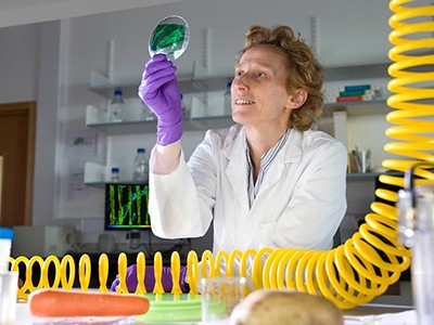
  • How to stop students cramming for exams? Send them to sea

    How to stop students cramming for exams? Send them to sea

    [ad_1]

    Nature, Published online: 30 April 2024; doi:10.1038/d41586-024-01209-y

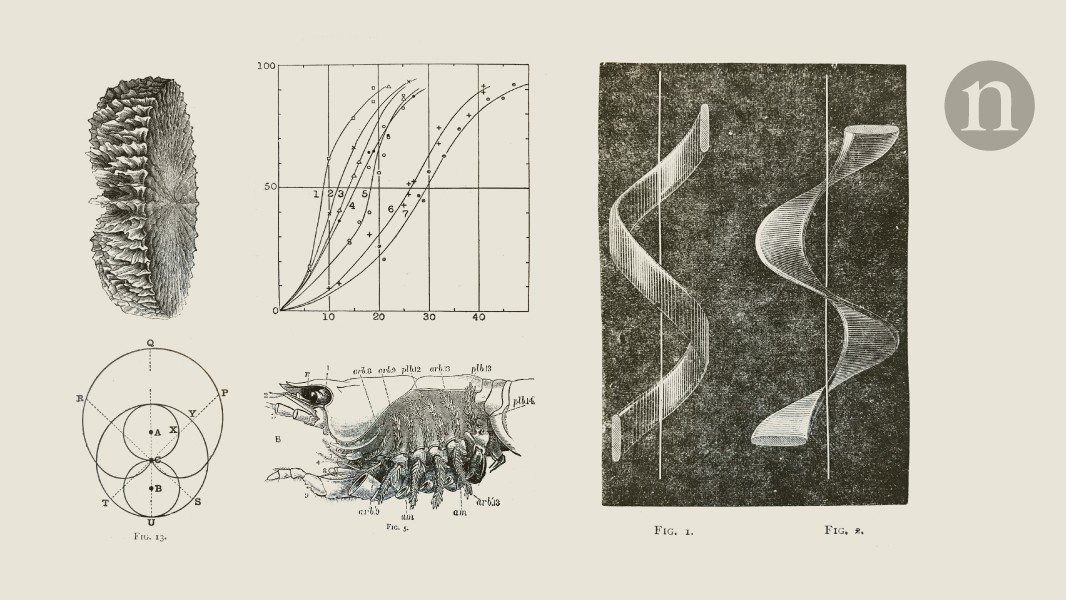
    An innovative proposal to stop exam over-preparation, plus William Bateson’s 1924 take on the previous century of biology, in the weekly dip into Nature’s archive.

    [ad_2]

    Source link

  • how Einstein lost the battle to explain quantum reality

    how Einstein lost the battle to explain quantum reality

    [ad_1]

    Quantum mechanics is an extraordinarily successful scientific theory, on which much of our technology-obsessed lifestyles depend. It is also bewildering. Although the theory works, it leaves physicists chasing probabilities instead of certainties and breaks the link between cause and effect. It gives us particles that are waves and waves that are particles, cats that seem to be both alive and dead, and lots of spooky quantum weirdness around hard-to-explain phenomena, such as quantum entanglement.

    Myths are also rife. For instance, in the early twentieth century, when the theory’s founders were arguing among themselves about what it all meant, the views of Danish physicist Niels Bohr came to dominate. Albert Einstein famously disagreed with him and, in the 1920s and 1930s, the two locked horns in debate. A persistent myth was created that suggests Bohr won the argument by browbeating the stubborn and increasingly isolated Einstein into submission. Acting like some fanatical priesthood, physicists of Bohr’s ‘church’ sought to shut down further debate. They established the ‘Copenhagen interpretation’, named after the location of Bohr’s institute, as a dogmatic orthodoxy.

    My latest book Quantum Drama, co-written with science historian John Heilbron, explores the origins of this myth and its role in motivating the singular personalities that would go on to challenge it. Their persistence in the face of widespread indifference paid off, because they helped to lay the foundations for a quantum-computing industry expected to be worth tens of billions by 2040.

    John died on 5 November 2023, so sadly did not see his last work through to publication. This essay is dedicated to his memory.

    Foundational myth

    A scientific myth is not produced by accident or error. It requires effort. “To qualify as a myth, a false claim should be persistent and widespread,” Heilbron said in a 2014 conference talk. “It should have a plausible and assignable reason for its endurance, and immediate cultural relevance,” he noted. “Although erroneous or fabulous, such myths are not entirely wrong, and their exaggerations bring out aspects of a situation, relationship or project that might otherwise be ignored.”

    To see how these observations apply to the historical development of quantum mechanics, let’s look more closely at the Bohr–Einstein debate. The only way to make sense of the theory, Bohr argued in 1927, was to accept his principle of complementarity. Physicists have no choice but to describe quantum experiments and their results using wholly incompatible, yet complementary, concepts borrowed from classical physics.

    In one kind of experiment, an electron, for example, behaves like a classical wave. In another, it behaves like a classical particle. Physicists can observe only one type of behaviour at a time, because there is no experiment that can be devised that could show both behaviours at once.

    Bohr insisted that there is no contradiction in complementarity, because the use of these classical concepts is purely symbolic. This was not about whether electrons are really waves or particles. It was about accepting that physicists can never know what an electron really is and that they must reach for symbolic descriptions of waves and particles as appropriate. With these restrictions, Bohr regarded the theory to be complete — no further elaboration was necessary.

    Such a pronouncement prompts an important question. What is the purpose of physics? Is its main goal to gain ever-more-detailed descriptions and control of phenomena, regardless of whether physicists can understand these descriptions? Or, rather, is it a continuing search for deeper and deeper insights into the nature of physical reality?

    Einstein preferred the second answer, and refused to accept that complementarity could be the last word on the subject. In his debate with Bohr, he devised a series of elaborate thought experiments, in which he sought to demonstrate the theory’s inconsistencies and ambiguities, and its incompleteness. These were intended to highlight matters of principle; they were not meant to be taken literally.

    Entangled probabilities

    In 1935, Einstein’s criticisms found their focus in a paper1 published with his colleagues Boris Podolsky and Nathan Rosen at the Institute for Advanced Studies in Princeton, New Jersey. In their thought experiment (known as EPR, the authors’ initials), a pair of particles (A and B) interact and move apart. Suppose each particle can possess, with equal probability, one of two quantum properties, which for simplicity I will call ‘up’ and ‘down’, measured in relation to some instrument setting. Assuming their properties are correlated by a physical law, if A is measured to be ‘up’, B must be ‘down’, and vice versa. The Austrian physicist Erwin Schrödinger invented the term entangled to describe this kind of situation.

    If the entangled particles are allowed to move so far apart that they can no longer affect one another, physicists might say that they are no longer in ‘causal contact’. Quantum mechanics predicts that scientists should still be able to measure A and thereby — with certainty — infer the correlated property of B.

    But the theory gives us only probabilities. We have no way of knowing in advance what result we will get for A. If A is found to be ‘down’, how does the distant, causally disconnected B ‘know’ how to correlate with its entangled partner and give the result ‘up’? The particles cannot break the correlation, because this would break the physical law that created it.

    Physicists could simply assume that, when far enough apart, the particles are separate and distinct, or ‘locally real’, each possessing properties that were fixed at the moment of their interaction. Suppose A sets off towards a measuring instrument carrying the property ‘up’. A devious experimenter is perfectly at liberty to change the instrument setting so that when A arrives, it is now measured to be ‘down’. How, then, is the correlation established? Do the particles somehow remain in contact, sending messages to each other or exerting influences on each other over vast distances at speeds faster than light, in conflict with Einstein’s special theory of relativity?

    The alternative possibility, equally discomforting to contemplate, is that the entangled particles do not actually exist independently of each other. They are ‘non-local’, implying that their properties are not fixed until a measurement is made on one of them.

    Both these alternatives were unacceptable to Einstein, leading him to conclude that quantum mechanics cannot be complete.

    Photograph taken during a debate between Bohr and Einstein

    Niels Bohr (left) and Albert Einstein.Credit: Universal History Archive/Universal Images Group via Getty

    The EPR thought experiment delivered a shock to Bohr’s camp, but it was quickly (if unconvincingly) rebuffed by Bohr. Einstein’s challenge was not enough; he was content to criticize the theory but there was no consensus on an alternative to Bohr’s complementarity. Bohr was judged by the wider scientific community to have won the debate and, by the early 1950s, Einstein’s star was waning.

    Unlike Bohr, Einstein had established no school of his own. He had rather retreated into his own mind, in vain pursuit of a theory that would unify electromagnetism and gravity, and so eliminate the need for quantum mechanics altogether. He referred to himself as a “lone traveler”. In 1948, US theoretical physicist J. Robert Oppenheimer remarked to a reporter at Time magazine that the older Einstein had become “a landmark, but not a beacon”.

    Prevailing view

    Subsequent readings of this period in quantum history promoted a persistent and widespread suggestion that the Copenhagen interpretation had been established as the orthodox view. I offer two anecdotes as illustration. When learning quantum mechanics as a graduate student at Harvard University in the 1950s, US physicist N. David Mermin recalled vivid memories of the responses that his conceptual enquiries elicited from his professors, whom he viewed as ‘agents of Copenhagen’. “You’ll never get a PhD if you allow yourself to be distracted by such frivolities,” they advised him, “so get back to serious business and produce some results. Shut up, in other words, and calculate.”

    It seemed that dissidents faced serious repercussions. When US physicist John Clauser — a pioneer of experimental tests of quantum mechanics in the early 1970s — struggled to find an academic position, he was clear in his own mind about the reasons. He thought he had fallen foul of the ‘religion’ fostered by Bohr and the Copenhagen church: “Any physicist who openly criticized or even seriously questioned these foundations … was immediately branded as a ‘quack’. Quacks naturally found it difficult to find decent jobs within the profession.”

    But pulling on the historical threads suggests a different explanation for both Mermin’s and Clauser’s struggles. Because there was no viable alternative to complementarity, those writing the first post-war student textbooks on quantum mechanics in the late 1940s had little choice but to present (often garbled) versions of Bohr’s theory. Bohr was notoriously vague and more than occasionally incomprehensible. Awkward questions about the theory’s foundations were typically given short shrift. It was more important for students to learn how to apply the theory than to fret about what it meant.

    One important exception is US physicist David Bohm’s 1951 book Quantum Theory, which contains an extensive discussion of the theory’s interpretation, including EPR’s challenge. But, at the time, Bohm stuck to Bohr’s mantra.

    The Americanization of post-war physics meant that no value was placed on ‘philosophical’ debates that did not yield practical results. The task of ‘getting to the numbers’ meant that there was no time or inclination for the kind of pointless discussion in which Bohr and Einstein had indulged. Pragmatism prevailed. Physicists encouraged their students to choose research topics that were likely to provide them with a suitable grounding for an academic career, or ones that appealed to prospective employers. These did not include research on quantum foundations.

    These developments conspired to produce a subtly different kind of orthodoxy. In The Structure of Scientific Revolutions (1962), US philosopher Thomas Kuhn describes ‘normal’ science as the everyday puzzle-solving activities of scientists in the context of a prevailing ‘paradigm’. This can be interpreted as the foundational framework on which scientific understanding is based. Kuhn argued that researchers pursuing normal science tend to accept foundational theories without question and seek to solve problems within the bounds of these concepts. Only when intractable problems accumulate and the situation becomes intolerable might the paradigm ‘shift’, in a process that Kuhn likened to a political revolution.

    The prevailing view also defines what kinds of problem the community will accept as scientific and which problems researchers are encouraged (and funded) to investigate. As Kuhn acknowledged in his book: “Other problems, including many that had previously been standard, are rejected as metaphysical, as the concern of another discipline, or sometimes as just too problematic to be worth the time.”

    What Kuhn says about normal science can be applied to ‘mainstream’ physics. By the 1950s, the physics community had become broadly indifferent to foundational questions that lay outside the mainstream. Such questions were judged to belong in a philosophy class, and there was no place for philosophy in physics. Mermin’s professors were not, as he had first thought, ‘agents of Copenhagen’. As he later told me, his professors “had no interest in understanding Bohr, and thought that Einstein’s distaste for [quantum mechanics] was just silly”. Instead, they were “just indifferent to philosophy. Full stop. Quantum mechanics worked. Why worry about what it meant?”

    It is more likely that Clauser fell foul of the orthodoxy of mainstream physics. His experimental tests of quantum mechanics2 in 1972 were met with indifference or, more actively, dismissal as junk or fringe science. After all, as expected, quantum mechanics passed Clauser’s tests and arguably nothing new was discovered. Clauser failed to get an academic position not because he had had the audacity to challenge the Copenhagen interpretation; his audacity was in challenging the mainstream. As a colleague told Clauser later, physics faculty members at one university to which he had applied “thought that the whole field was controversial”.

    Alain Aspect, John Clauser and Anton Zeilinger seated at a press conference.

    Aspect, Clauser and Zeilinger won the 2022 physics Nobel for work on entangled photons.Credit: Claudio Bresciani/TT News Agency/AFP via Getty

    However, it’s important to acknowledge that the enduring myth of the Copenhagen interpretation contains grains of truth, too. Bohr had a strong and domineering personality. He wanted to be associated with quantum theory in much the same way that Einstein is associated with theories of relativity. Complementarity was accepted as the last word on the subject by the physicists of Bohr’s school. Most vociferous were Bohr’s ‘bulldog’ Léon Rosenfeld, Wolfgang Pauli and Werner Heisenberg, although all came to hold distinct views about what the interpretation actually meant.

    They did seek to shut down rivals. French physicist Louis de Broglie’s ‘pilot wave’ interpretation, which restores causality and determinism in a theory in which real particles are guided by a real wave, was shot down by Pauli in 1927. Some 30 years later, US physicist Hugh Everett’s relative state or many-worlds interpretation was dismissed, as Rosenfeld later described, as “hopelessly wrong ideas”. Rosenfeld added that Everett “was undescribably stupid and could not understand the simplest things in quantum mechanics”.

    Unorthodox interpretations

    But the myth of the Copenhagen interpretation served an important purpose. It motivated a project that might otherwise have been ignored. Einstein liked Bohm’s Quantum Theory and asked to see him in Princeton in the spring of 1951. Their discussion prompted Bohm to abandon Bohr’s views, and he went on to reinvent de Broglie’s pilot wave theory. He also developed an alternative to the EPR challenge that held the promise of translation into a real experiment.

    Befuddled by Bohrian vagueness, finding no solace in student textbooks and inspired by Bohm, Irish physicist John Bell pushed back against the Copenhagen interpretation and, in 1964, built on Bohm’s version of EPR to develop a now-famous theorem3. The assumption that the entangled particles A and B are locally real leads to predictions that are incompatible with those of quantum mechanics. This was no longer a matter for philosophers alone: this was about real physics.

    It took Clauser three attempts to pass his graduate course on advanced quantum mechanics at Columbia University because his brain “kind of refused to do it”. He blamed Bohr and Copenhagen, found Bohm and Bell, and in 1972 became the first to perform experimental tests of Bell’s theorem with entangled photons2.

    French physicist Alain Aspect similarly struggled to discern a “physical world behind the mathematics”, was perplexed by complementarity (“Bohr is impossible to understand”) and found Bell. In 1982, he performed what would become an iconic test of Bell’s theorem4, changing the settings of the instruments used to measure the properties of pairs of entangled photons while the particles were mid-flight. This prevented the photons from somehow conspiring to correlate themselves through messages or influences passed between them, because the nature of the measurements to be made on them was not set until they were already too far apart. All these tests settled in favour of quantum mechanics and non-locality.

    Although the wider physics community still considered testing quantum mechanics to be a fringe science and mostly a waste of time, exposing a hitherto unsuspected phenomenon — quantum entanglement and non-locality — was not. Aspect’s cause was aided by US physicist Richard Feynman, who in 1981 had published his own version of Bell’s theorem5 and had speculated on the possibility of building a quantum computer. In 1984, Charles Bennett at IBM and Giles Brassard at the University of Montreal in Canada proposed entanglement as the basis for an innovative system of quantum cryptography6.

    It is tempting to think that these developments finally helped to bring work on quantum foundations into mainstream physics, making it respectable. Not so. According to Austrian physicist Anton Zeilinger, who has helped to found the science of quantum information and its promise of a quantum technology, even those working in quantum information consider foundations to be “not the right thing”. “We don’t understand the reason why. Must be psychological reasons, something like that, something very deep,” Zeilinger says. The lack of any kind of physical mechanism to explain how entanglement works does not prevent the pragmatic physicist from getting to the numbers.

    Similarly, by awarding the 2022 Nobel Prize in Physics to Clauser, Aspect and Zeilinger, the Nobels as an institution have not necessarily become friendly to foundational research. Commenting on the award, the chair of the Nobel Committee for Physics, Anders Irbäck, said: “It has become increasingly clear that a new kind of quantum technology is emerging. We can see that the laureates’ work with entangled states is of great importance, even beyond the fundamental questions about the interpretation of quantum mechanics.” Or, rather, their work is of great importance because of the efforts of those few dissidents, such as Bohm and Bell, who were prepared to resist the orthodoxy of mainstream physics, which they interpreted as the enduring myth of the Copenhagen interpretation.

    The lesson from Bohr–Einstein and the riddle of entanglement is this. Even if we are prepared to acknowledge the myth, we still need to exercise care. Heilbron warned against wanton slaying: “The myth you slay today may contain a truth you need tomorrow.”

    [ad_2]

    Source link

  • Las Boriqueñas remembers the forgotten Puerto Rican women who tested the first pill

    Las Boriqueñas remembers the forgotten Puerto Rican women who tested the first pill

    [ad_1]

    Guadalís Del Carmen, Maricelis Galanes, Ashley Marie Ortiz, & Nicole Betancourt in Las Borinqueñas.

    Las Borinqueñas explores how women sought control of their reproductive lives in the 1950s.Credit: Valerie Terranova

    Las Borinqueñas Directed by Rebecca Aparicio Ensemble Studio Theatre, New York City 3 April – 5 May 2024

    It’s the 1950s and two US scientists are looking for somewhere to test the first birth-control pill. Where better than Puerto Rico? The territory had an established network of family-planning clinics, and the use of contraception had been legal there since 1937. That wasn’t the case in much of the United States, including Massachusetts, where biologist Gregory Pincus and obstetrician-gynaecologist John Rock were developing the oral contraceptive.

    Puerto Rican women were interested in a pill that could give them more control over their reproductive lives. But as they lined up outside a clinic in the outskirts of San Juan to receive the medication, many were unaware that it was an experimental drug and they were part of a clinical trial. When some of them started reporting debilitating side effects, these were dismissed as psychosomatic.

    The play Las Borinqueñas, whose title means ‘the Puerto Rican women’, revisits the complicated history of the world’s first oral contraceptive. Mixing the excitement of scientific breakthrough with the shock of flawed research ethics and shadows of colonialism and exploitation, it puts the spotlight on the women who, after playing a key part in the pill’s development, were quickly forgotten.

    It’s a long-overdue tribute and, most importantly, a reminder to remain vigilant against abuse and disrespect in studies involving human participants. In a world where the fight for access to birth control is ongoing, it is bold and commendable to recognize that this significant advance was built on ethically problematic studies that harmed some of the very women they aimed to serve and empower.

    Written by Nelson Diaz-Marcano, a Puerto Rican theatre-maker based in New York City, the show was developed by the Ensemble Studio Theatre and the Alfred P. Sloan Foundation, a research funder also based in the city. It had its world premiere on 3 April and is playing until 5 May at the Ensemble Studio Theatre in New York City.

    Taking control

    The play follows the intertwined lives of five women — Chavela, Yolanda, Fernanda, Maria and Rosa — as they cross paths with the researchers testing the pill. As the audience witnesses their love stories, aspirations, struggles and loyal friendships, the protagonists open a window on the lives of hundreds of Puerto Rican women who enrolled in the tests, and how the experience changed them.

    Each character is affected in a different way. Chavela sees the trial as chance to slow down the growth of her family while maintaining a passionate marriage. Yolanda envisions it as the lifeline that might save other women from the fate of her sister, Fernanda, who dies as a result of an illegal abortion. For Maria, it’s about avoiding pregnancy to advance her dream of becoming a writer — and about honouring Fernanda, her soulmate, with whom she could never openly have a relationship because of societal norms. But the hope brought on by the pill slowly fades when the women start feeling unwell.

    Hanna Cheek & Helen Coxe in Las Borinqueñas.

    The play shows how researchers and trial facilitators played down side effects because of the pill’s ground-breaking implications.Credit: Valerie Terranova

    Rosa, who was suspicious of the pill from the start, urges the others to stop taking it, while boasting about the benefits of the sterilization that she underwent after giving birth. The doctors who suggested the procedure, however, never told her it was irreversible. The heartbreaking scene when she learns she will never be able to have another baby signals that the clinical trial wasn’t the first instance of medical abuse these women endured. By 1953, a eugenics-based programme in Puerto Rico had led to the sterilization of nearly one-fifth of women on the island to address concerns about ‘surplus population’.

    From rabbits to women

    The birth-control pill was the result of the encounter of Pincus and Rock, who were both studying the effects of synthetic progesterone, but in different contexts. Pincus was looking into the anti-ovulatory effect of the hormone in rabbits, and Rock was exploring it as a means to treat his patients’ infertility. The play focuses on Pincus, portrayed as an ambitious scientist determined to carve his name into history by creating a revolutionary product.

    When someone becomes pregnant, their levels of progesterone go up, signalling to the body to shut down the ovaries and not release new eggs. Whereas Pincus wanted to mimic this process for the purpose of contraception, Rock hoped that a pause in ovulation would allow his patients’ reproductive systems to reset, increasing their chances of pregnancy after the treatment.

    The scientists came together to test the pill in humans. The play briefly refers to a couple of small trials done in the United States, but to get the pill approved, it had to be tested on a larger scale. Pincus sets his sights on Puerto Rico and seeks to partner with Edris Rice-Wray, who was then the medical director of the Family Planning Association of Puerto Rico.

    Rice-Wray expresses her concerns about negative side effects that had been observed in previous tests, but is convinced to join the project by Pincus’s wife, who highlights the potentially revolutionary implications of the pill for women around the world.

    Rice-Wray is portrayed as a responsible public-health official who is nonetheless persuaded to push the boundaries of ethics for the greater good. She launches the programme with fanfare in 1956 and, at the suggestion of Pincus, does not mention the potential side effects to participants, most of whom are poor women with little access to health care. Her discomfort with the omission increases as she hears that the trial is taking a toll on participants.

    In one scene, Chavela is taking laundry from the line when she is struck by dizziness and nausea. Her sister Rosa warns her that the pill is to blame, but she prefers to continue taking it rather than to risk becoming pregnant again. Rice-Wray reports those concerns to Pincus, who minimizes them as minor inconveniences compared with the wider benefits of the drug. Because of his disregard for the Puerto Rican study participants, the real-life Pincus was later accused of colonialism and exploitation of women of colour.

    The protagonists eventually stop taking the pill and don’t experience long-term consequences. But the play mentions that three Puerto Rican women died during the trial, and that their deaths were never investigated.

    Trial and error

    In reality, of around 800 women who enrolled in the study, only 130 took the pill for a year or more, most dropping out because of the side effects. To make the results look more impressive, Pincus described them by saying that no pregnancy had been registered “in the 1,279 menstrual cycles” during which the treatment had been followed. In the play, his character brushes off the accusation of data embellishment. For him, it was simply a matter of using a different metric.

    The pill, branded as Enovid, went on to be approved by the US Food and Drug Administration as a contraceptive in 1960. The participants of the clinical trial didn’t have access to the product once it reached the market: the price was prohibitive for the Puerto Rican working class.

    More than six decades later, the contraceptive pills available are much safer. But access is still an issue. In the United States, until last year, people still needed a prescription to buy oral contraceptives — a significant barrier for those without health insurance.

    Las Borinqueñas concludes with the women refusing to be defined by the experience of being exploited by scientists and having their right to decide about their own reproductive lives stripped away. Rosa publicly denounces the pill’s side effects and the irreversibility of sterilization on a radio show; she also conveys her resilience and hope for the future. The women will continue to take care of their families, to work and to pursue their dreams. They celebrate life and laugh at adversity.

    Some would argue that their suffering was a small price to pay for the wider impacts of pill. But by giving names to the study participants and telling their stories, Las Borinqueñas serves as a powerful reminder that such disregard and injustice was never acceptable.

    [ad_2]

    Source link

  • Network of large pedigrees reveals social practices of Avar communities

    [ad_1]

    Ancient-DNA laboratory analyses

    For the archaeogenetic investigations, petrous bones and teeth were preferentially sampled (Supplementary Table 1). Samples were prepared in dedicated ancient-DNA laboratory facilities at the HUN-REN RCH Institute of Archaeogenomics in Budapest. Sample surfaces were decontaminated using UVC light and cleaned by mechanical removal. About 25–50 mg bone powder was obtained by drilling or powdering and transferred to MPI-EVA in Leipzig, Germany. DNA extraction and subsequent laboratory steps were done in the Ancient DNA Core Unit of the MPI-EVA. DNA was extracted from between 25 mg and 52 mg of powdered sample material using a silica-based method optimized for the recovery of short DNA fragments35. Briefly, lysates were prepared by adding 1 ml extraction buffer (0.45 M EDTA, pH 8.0, 0.25 mg ml–1 proteinase K, 0.05% Tween-20) to the sample material in 2.0-ml Eppendorf LoBind tubes and rotating the tubes at 37 °C for approximately 16 h35,36. Using an automated liquid-handling system (Bravo NGS Workstation B, Agilent Technologies), DNA was purified from 150 µl lysate using silica-coated magnetic beads and binding buffer D, as described previously36. Elution volume was 30 µl. Extraction blanks without sample material were carried alongside the samples during DNA extraction.

    DNA libraries were prepared from 30 µl extract using an automated version of single-stranded DNA-library preparation37 described in detail previously38. Escherichia coli uracil–DNA–glycosylase (UDG) and E. coli endonuclease VIII were added during library preparation to remove uracils from the interior of molecules. Libraries were prepared from both the sample DNA extracts and the extraction blanks, and further negative controls (library blanks) were added. Library yields and efficiency of library preparation were determined using two quantitative PCR assays38. Libraries were tagged with pairs of sample-specific indices by PCR extension using AccuPrime Pfx DNA polymerase as described previously38. Indexed libraries were amplified and purified using SPRI (solid-phase reversible immobilization) technology39 as described previously38.

    Sample and control libraries were enriched in solution for 1,237,207 informative SNPs (a method commonly used in the field and known as 1240k capture40) targeting 394,577 SNPs first reported in ref. 41 (390k panel) and 842,630 SNPs first reported in ref. 42 (840k panel). Two consecutive rounds of 1240k capture were performed using the Bravo NGS workstation B. Up to 20 libraries were pooled together and sequenced single-read or pair-read on a HiSeq4000 sequencing platform (Illumina Technology). In total, 440 1240k-enriched libraries were sequenced and an average coverage of 2.6× (median 2.25×) for the 1,237,207 sites in the genome, corresponding to a median of 708,514 1240k SNPs covered at least once (Supplementary Table 1).

    Ancient-DNA data process and quality controls

    The raw sequenced read data (fastq files) were processed through a nf-core/eager v.2.3.2 pipeline43 (https://nf-co.re/eager). To remove adaptors and short reads of less than 30 base pairs, AdapterRemoval v.2.3.1 was used44. The reads were then mapped to the Human Reference Genome Hs37d5 using the bwa v0.7.17 aln/samse alignment algorithm45 with the parameters -n and -l set to 0.01 and 1,024, respectively. The reads with phred mapping quality of less than 30 were then discarded using -q (q30-reads) in Samtools v1.9 (ref. 46). We then used the Picard tools MarkDuplicates function (https://github.com/broadinstitute/picard) to remove PCR duplicates. To estimate the amount of cytosine-to-thymine taphonomic deamination at the ends of the mapped fragments, we used mapDamage v.2.0 (ref. 47) run on a subset of 100,000 q30 reads. Exogenous human autosomal DNA contamination was estimated in male individuals by assessing X-chromosome heterozygosity levels using ANGSD v.0.910 (ref. 48) and mtDNA contamination in male and female individuals was estimated using Schmutzi49. Schmutzi was also used to reconstruct the consensus mitochondrial genome sequence of each individual used as input for HaploGrep2 (ref. 50) to assign mitochondrial haplogroups. For the purpose of graphical representation in Extended Data Fig. 4, all the mitochondrial haplogroups were pruned to the first three characters. If two individuals had, respectively, a two- and three-characters resolution, both of their haplogroups were trimmed to the first two characters. Individuals with only a one-character resolution were excluded from the plot.

    Y-chromosome haplogroups were inferred using two different methodologies and the results compared. The Y-chromosome variants were called from in the bam files from samples whose genetic sex was estimated to be male or unassigned using the Samtools v1.946 mpileup and PileupCaller (https://github.com/stschiff/sequenceTools) using the mode –majorityCall; Y-chromosome haplogroup assignment was performed using the software yHaplo (https://github.com/23andMe/yhaplo), with ISOGG panel v.11.349 as a reference (https://isogg.org/tree/; date of access: 2 February 2023). Y-chromosome haplogroups were also defined using the Y-Lineage-Tracker subcommand ‘classify’51, using as a reference panel the ISOGG Y-haplogroup tree v.15.73 (https://isogg.org/tree/); in this case the input files were genotypes from each individual, estimated using the allelePresence method from the ATLAS (https://bitbucket.org/wegmannlab/atlas/)52 call tool, accounting for post-mortem damage patterns and base-score recalibration patterns, estimated respectively with the ATLAS tools PMD and recal.

    The results from the two methodologies were then compared, taking into account the differences between the two reference panels. In cases where the two methodologies yielded deeply diverging results (that is, to the first two ISOGG alphanumeric classification symbols) or were discordant with the estimated reciprocal genetic relatedness between individuals (described in the Biological relatedness section), the haplogroup assessment was further investigated using the software pathPhynder53 with default options, using as reference the BigTree Y-chromosome dataset and the reference phylogenetic tree for sample placement provided by GitHub with the software and as input files the bam files filtered for phred mapping quality more than 30. In any other case, the conservative results from Y-LineageTracker (the column Key haplogroup) were considered reliable, given the more-stringent estimation of the genotypes and the updated ISOGG Y-chromosome phylogenetic tree version.

    The results of the whole procedure can be found in Supplementary Table 1. PileupCaller (https://github.com/stschiff/sequenceTools) was used to carry out genotype calling from the q30 reads with the –randomHaploid flag that calls haploid genotypes by randomly choosing one high-quality base (phred base quality score ≥30) on the 1240k panel (pseudodiploid calls). We also used the –singleStrandMode, which removes only real cytosine-to-thymine deamination observed with single-stranded DNA libraries by ignoring cytosine–thymine polymorphisms at reads aligning to the forward strand and guanine–adenine polymorphisms at reads aligning to the reverse strand.

    To produce the Y-chromosome haplogroup plots in Extended Data Fig. 4, all the haplogroup nomenclature was pruned to the first three characters; haplogroups with less than three characters of ISOGG notation were excluded from the plots. Complete Y-chromosome haplogroups can be found in Supplementary Table 1.

    We found low mitochondrial contamination estimates (Supplementary Table 1). Most were less than 5% and only five samples had values between 5% and 10%. Of these we excluded one female individual (RKF048) with 7% contamination and one individual (KFJ019) with 5% contamination and ambiguous sex determination (an indirect sign of possible contamination); the remaining male individuals had low nuclear contamination and were therefore kept for nuclear genomic analyses. We also found low nuclear contamination estimates among the male individuals. We excluded four further individuals with values of more than 7%; RKF094 (15% contamination) was still counted among the related as showing high likelihood of close genetic relatedness with other individuals (Supplementary Table 4). We also excluded individuals with particularly low coverage (more than 20,000 SNPs) because they were not practically usable for further analyses (additional filtering for higher coverage thresholds is detailed for specific analyses in the following sections); these include two individuals also excluded for contamination and another 15 individuals still included as showing high likelihoods of close relatedness (RKF225, HNJ005, HNJ009 and RKF128). We kept 419 individuals for further analyses, 413 excluding one pair among the identical pairs found, and 424 including the previously published individuals from the KUP and KFJ sites10 (Supplementary Table 1). We then merged them with a reference genome-wide panel of 2,280 modern individuals genotyped with microarray technology using the commercial HumanOrigins chip54,55,56 and previously published ancient-individuals’ genotypes sequenced with the same 1240k capture method or a 1240k SNPs subset from data obtained using whole-genome shotgun sequencing10,27,54,55,57,58,59,60,61,62,63,64,65,66,67,68,69,70,71,72,73,74 downloaded from Poseidon (https://poseidon-framework.github.io). We produced two datasets, one including the modern data and the SNPs overlap between the 1240k sites and the HumanOrigins SNP chip (1240KHO dataset, around 600,000 SNPs), and one with ancient data and the whole 1240k panel (the 1240k dataset).

    Genomic ancestry modelling with PCA, qpWave/qpAdm, DATES

    We used principal component analysis (PCA) with smartpca v.16000 in the EIGENSOFT v.6.0.1 package75 on the 1240KHO dataset using the lsqproject and the autoshrink parameters to project the genotypes of the ancient individuals (containing variable amounts of missing data) on top of the principal components calculated on the set of modern worldwide populations. For one PCA (Fig. 4a) we used a subset of Eurasian populations (the Eurasian PCA) as originally in reference54 adapted as in reference27, and for another PCA (Extended Data Fig. 8b) we used a standard subset of only west Eurasian populations (the west Eurasian PCA), as originally reported76 and then adapted10.

    We used the software qpWave/qpAdm (v.1520) of the ADMIXTOOLS package56 to run the f4-statistics-based ancestry analyses on the 1240k dataset41,77. Standard errors for the computed f-statistics were estimated using a block jack-knife with a 5-cM block. We used the default allsnps: NO parameter, thereby calculating all the underlying f4-statistics using the SNP overlap between all the groups for each test. We used a set of outgroups (or right populations) that are similar to those of a previous study10 that included representatives of ancient Eurasian lineages (European Mesolithic hunter-gatherers, European/Anatolia Neolithic, Levant Neolithic, Iranian Neolithic for western Eurasia, and ancient North Eurasian lineage (ANE76), ANA, ancient Siberian and southern East Asia for eastern Eurasia, and key non-Eurasian ones (African, South Asian, Native American) when available, otherwise hte present-day proxies Mbuti.DG, Levant_N, Onge.DG, Iran_N, Iron_Gates_HG, EHG, Mixe.DG, Anatolia_N, DevilsCave_N.SG, Tarim_EMBA1, Kolyma_M.SG and YR_LN. The only difference with respect to ref. 10 is that we used Tarim_EMBA1 (ref. 72) instead of the three Russia_Bolshoy individuals65, which is a higher-coverage dataset of 12 individuals and a better representative of the ANE lineage73 than any other high-ANE ancestry group available in the literature.

    To select the sources (or left populations) to model the admixed ancestry of our newly sequenced individuals (the targets), we followed the following rationale. Among the data available from previous studies, we selected only ancient populations (of more than two individuals) that are either approximately contemporaneous or temporally preceding but are as close as possible to the time period of our target individuals, as suggested previously78. In our selection, we also considered the findings from a previous genomic study of the Avar period10, as well as populations that are geographically, historically and archaeologically relevant. This led to a selection of 13 different source groups falling in 3 categories. (1) Sources representative of the east Eurasian Steppe ancestry that include ancient populations and cultures available from preceding time periods in the east Eurasian Steppe and surrounding areas in east Asia. (2) ‘Pre-Avar’ populations that are found in the Carpathian Basin in the first centuries ad, before the Avar period. (3) Relevant temporally preceding (first millennia bc and ad) populations available from across the Pontic- and central Asian Steppe (the ‘steppe’ sources).

    Two- and three-way combinations of these sources led to a total of 190 different combinations being tested, all with qpWave P-values of much less than 0.05, which means that the sources are sufficiently differentiated with respect to the set of outgroups. They are therefore suitable sources to be tested76 (Supplementary Table 5), applying the following rationale, which is the same as that used in a previous study10 based on suggestions discussed previously78. We first tested two-way admixing sources using all combinations of eastern Eurasian Steppe groups plus the pre-Avar and steppe sources. If we could reject one but not the other, between the pre-Avar and steppe source models (if one had P < 0.05 we can reject; if the other had P  >  0.05 we cannot reject), we considered the one we cannot reject (P  >  0.05) as valid. If the two-way models did not significantly reject one or the other between the pre-Avar and steppe sources (both with P  >  0.05) or produced no fitting results at all (both with P   < 0.05), we proceeded by testing three-way competitive models, including the eastern Eurasian populations and contrasting directly the pre-Avar plus steppe sources as well as pre-Avar plus pre-Avar, accounting for the variability in ancestry and time period between the pre-Avar populations.

    If the three-way models resulted in one of the two contrasting sources between pre-Avar plus steppe resetting the other (bringing its estimated admixture proportion to 0%), we considered these models. If the contrasting sources had intermediate admixture proportions, we considered as successful only those tests that could reject one of the two scenarios between either pre-Avar plus steppe or pre-Avar plus pre-Avar. The individuals who still had unresolved or non-fitting models between a pre-Avar or a steppe source were considered unsolved or failed and were not used for further meta-analyses or interpretations.

    For the sake of simplicity and consistency, we chose one eastern Eurasian source to include in our plots and summary statistics: the genetically easternmost group of individuals from the early Avar period in the DTI region (DTI_EA_East; Fig. 4 and previously published10), to which we added data from unrelated individuals at the early-period site of KUP that presented the same genomic profile (Supplementary Fig. 12). We always used this eastern proxy, except in the few instances in which it did not produce fitting models, in favour of another one, suggesting an existing heterogeneity in the eastern component although much reduced with respect to the variability in the western sources (Supplementary Table 5). Nevertheless, it is important to note that although DTI_EA_East is the source that overall produced more fitting models, several other eastern sources (including lateXiongnu, AR_Xianbei_P_2c) resulted in many equally fitting models as well (Supplementary Table 5).

    We used DATES v.753 (https://github.com/priyamoorjani/DATES) to date the average time of the east–west Eurasian ancestry admixture estimated for most of the Avar period individuals from the four sites analysed. This method is based on the same principle as many admixture dating methods70,79; it assumes an admixture event between two admixing source populations, an east Asian and a west Eurasian one; in our case we used the unadmixed and high-SNP-covered LBA/IA group of the Ulaanzuukh_SlabGrave in Mongolia63 or the same DTI_EA_East group used in the main qpAdm models as an ANA proxy and the pre-Avar Carpathian Basin ancient sources, Sarmatian10 and Longobard period58 individuals, as a west Eurasian ancestry proxy. DATES calculates the decay of ancestry covariance coefficients between every pair of available overlapping SNPs between the test individuals and the source populations over increasing-genetic-distance windows70. Population-genetic theory suggests that if admixture happens, an exponential function can be fitted to the decay of weighted ancestry covariance, and the number of generations since admixture can be derived from the parameters of such functions79. The higher age limit of admixture events that would still produce detectable decays is theoretically considered to be around 4,000 years80. In practice, recent admixture events (about one to three generations ago) are not properly detected because chromosomal recombination had insufficient generation time to start producing the expected decay pattern81,82. To estimate the goodness of a fit, DATES calculates standard errors and Z-scores using a jack-knife approach, dropping a chromosome at a time. We set a maximum distance parameter of 0.5 cM, a bin size of 0.001 and a starting genetic distance of 0.45 cM. The integrated least-square function was used to estimate the number of generations since admixture parameter. If the raw data show no decay, the exponential function either cannot be fitted or is fitted with low Z-scores, much less than 2, and unreasonable dating estimates with negative values, or large numbers over the theoretical maximum of 4,000 years back in time. All samples showing such values were also inferred as non-admixed by PCA and qpAdm and were excluded from our inferences. For Extended Data Fig. 9, we also included dates with Z-scores of less than 2 (shown with a transparency factor) because in part they reflect the recent (for example, first or second generation) admixture events that we can observe directly in the pedigrees. These DATES estimates are mostly not significant because there is no decay pattern yet to fit an exponential function, but some still provide qualitatively correct recent admixture dates (Supplementary Table 1). We used a standard of 29 years per generation70 to convert the generation times in years since admixture, and used the Avar-period chronological phase of the individuals as the date at death.

    Biological relatedness

    We used KIN16 as the primary method to assess biological relatedness between each pair of individuals from the four sites we investigated, although we validated the relatedness estimates with the independent methods of haplotype-IBD (detailed below) and BREAD (https://github.com/jonotuke/BREADR) (Supplementary Information). Given that single-stranded UDG-half treated libraries still preserve a roughly 10–30% proportion of C-to-T deamination at the last two base pairs of the mapped fragments, for this analyses we masked two base pairs at both ends of the q30 reads using the trimBam module of bamUtil v.1.0.13 (ref. 83) and used these masked bam files as input data. KIN can confidently identify first- and second-degree relations while differentiating between parent–child and sibling relations16. Although the method does not explicitly differentiate relationships within the second degree, it outputs information about IBD sharing that can help to differentiate between avuncular and grandparent–grandchild relationships. We simulated avuncular, half-sibling and grandparent–grandchild pairs (Supplementary Information) to show that the length of IBD segments and the number of IBD segments can be used to differentiate between avuncular and grandparent–grandchild relationships, while half siblings overlap with both cases. Furthermore, KIN provides indications about third-degree relationships (with around 70% accuracy at 4× sequence coverage). Although these analyses are not sufficient to confidently identify within second-degree relationships, and may lack the power to identify third-degree relatives, they can be crucial when combined with other information, such as pedigree information from different pairs as well as from information about the skeletal age at death, the sex and the uniparental haplogroups (Y chromosome and mtDNA). Therefore, all this information was considered when building and cross-checking the pedigrees of biological relatedness (Supplementary Information). For clarity, we numbered the pedigrees that we found and we define one pedigree as a group of individuals who can be directly connected with close genetic relatedness and for whom a line of descent can be traced. In the case of the largest pedigree we reconstructed (146 individuals from RK), we divided it into five pedigrees descending from five different groups of 11 ‘founder male individuals’ (including multiple brothers as co-founders).

    Simulations on second-degree relationships

    We followed the methods section for KIN16 and simulated eight diploid individuals using msprime84 with default parameters for the mutation rate (1 × 10–8 per base per generation), the recombination rate r (1 × 10–8 per base per generation) and an effective population size of 3,000. For each individual, we simulated 22 chromosomes with the same lengths as the GRCh38.p14 genome. To form a pedigree, we first simulated a recombined set of chromosomes for each parent and combined them to create the progeny. We obtained recombination points for each chromosome from the software Ped-sim85. We matched the genotype density and the coverage of reads to that of our samples. We simulated 60 such pedigrees (see figure S9 in ref. 16 and Supplementary Figs. 17 and 18).

    Consanguinity test (ROHs)

    Consanguinity can be tested genetically by a straightforward approach: counting the length and number of long stretches of homozygous portions along the genome of an individual. This analysis is usually defined as ROHs. To estimate ROH, we applied a method called hapROH86 that was designed to infer them on pseudo-haploid, lower-coverage and higher-missing-data ancient DNA samples; the method has also been shown empirically to be highly consistent with independent ROH estimates calculated on the same ancient imputed diploid genomes10. Specific patterns of long ROH (more than 4 cM) along the genome of an individual are typical of consanguineous unions between some of its recent ancestors (up to second-degree cousins86). In Extended Data Fig. 5 we plotted ROH using the python package implemented in hapROH (https://pypi.org/project/hapROH/).

    Genotype likelihood calls and imputation/phasing

    Haplotype-based analyses (such as IBD described below) require information of the phase for each pair of paternal and maternal chromosomes of an individual, and this in turn requires there to be virtually no missing data along the genome. Obtaining such data from ancient genomes has been shown by recent studies87,88 to be reliable in other similar contexts for coverage of more than 0.5–0.7×, and it has also been applied to 1240k capture data10,89 through simultaneous statistical imputation and phasing. We used the ancient-DNA-specific genotype caller MLE function of ATLAS (https://bitbucket.org/wegmannlab/atlas/)52 to call genotype likelihoods. ATLAS can also calculate the base-quality recalibration (the recal function) that we performed in batches among libraries sequenced in the same sequencing run, accounting for specific sequencing errors. ATLAS recalibration also corrects the base qualities accounting for the empirical ancient DNA-damage pattern observed from the data and reduces the effect of reference bias introduced by genome mapping by relying on a list of 10 million highly conserved genomic positions across 88 mammal species downloaded from ensembl (https://grch37.ensembl.org/). We called genotype likelihoods on the whole 1,000-genomes SNPs panel of around 20 million SNPs and used these calls as input data for imputation with GLIMPSE90, for which we used the phased 1,000 genomes phase-3 release data as reference haplotypes91. We ran GLIMPSE with the default parameters using sex-averaged genetic maps from HapMap, as suggested previously88. The function GLIMPSE_phase was used to perform simultaneous imputation and phasing on genomic chunks of 2,000,000 base pairs with a buffer of 200,000 base pairs. We then used the integrated GLIMPSE_ligate and GLIMPSE_sample functions and bcftools v1.3 (refs. 88,92) to obtain the final phase/imputed vcf files with the genotypes posterior probabilities at every 1240k position.

    Haplotype IBD sharing analysis

    We performed haplotype IBD analysis with ancIBD, a recently developed method that accounts for the high phasing errors of ancient DNA93. This analysis searches for long haploid blocks along the genomes of two individuals that are identical by descent (IBD), meaning they have been inherited by a common ancestor at some time in the past. Therefore, it can detect close genetic relatives (first to third degrees of relation) as KIN does, but it can also detect more-distant relations, up to sixth degree, within ranges of biological stochasticity85. However, it requires a much higher threshold of coverage, reducing the number of individuals analysed relative to KIN. We used imputed or phased data, including only those individuals with more than 450,000 SNPs obtained with our pseudo-haploid calls and SNPs with genotype posterior probabilities greater than 0.99 after imputation. We used the HapBLOCK function of ancIBD to perform the pairwise estimation with default parameters and only shared blocks of more than 8 cM containing more than 220 SNPs per centimorgan were considered. To further filter for possible false-positive hits, we considered only shared IBD segments longer than 12 cM, and if a pair of individuals had segments of less than 16 cM, we included them only if they had more than one such segment (Supplementary Table 4). We used Cytoscape v.3.9.1 (ref. 94) to plot the networks of pairwise IBD relations.

    Network analysis

    For the IBD network analysis, only the Avar-period individuals were included. Because subadult individuals might be a confounding factor when assessing the sex-specific patterns of mobility and connectedness, we made an additional network that included only adults. The threshold of adulthood was set at 18 years of age, based on the lower limit of the estimated age of the youngest parent. The entire network consisted of 257 nodes, of which 195 represented adults (105 male and 90 female individuals) and 62 subadults (35 male and 27 female individuals) from four archaeological sites. The links of the network are represented by the IBD connections, which number 2,658 if the entire network is considered and 1,211 if only the adults are selected (Supplementary Table 4). In our analysis, we considered both unweighted and weighted networks. The unweighted network represents a configuration in which the found IBD relations define the presence or absence of links irrespective of their values. However, in the weighted network, the links are weighted by the maximum IBD values of the analysis, allowing the magnitude of relatedness to be evaluated. Both networks are undirected because sharing of IBD segments between two individuals has no directionality.

    Degree centrality (k) is defined as the number of links held by the node. The average degree k of the Avar-period adults’ network is 18.07. Considering the assigned weights on the links, which in our case is the sum of the weights (max_IBD) of the links attached to each node, the mean strength w is 1,620.54. When sex is considered as a node attribute, the degree and the strength distributions are significantly different between male and female individuals (Fig. 3c and Supplementary Figs. 47 and 48). For male individuals, k is 27.39 and w is 2,392.37, whereas for female individuals, k is 7.21 and w is 720.08. The two-sample Kolmogorov–Smirnov test revealed significant differences between the male and female individuals’ degree and strength distribution (P < 0.05).

    The degree centrality of a node can be partitioned into within-module (kW) and between-module (kB) links by considering the archaeological site of the burial as a module. The kB/k ratio represents the ratio of between-module connections over the total connections, which can range between 0 and 1, with 0 indicating that related individuals are buried solely at the same site and 1 indicating that related individuals are buried only at a different site. To evaluate this ratio, the value of degree centrality must also be considered because individuals with small degree centrality may have a higher kB/k ratio. The other results of the analysis are explained in Supplementary Figs. 44–48. The analysis was performed using R and the node measurements were calculated using customized R scripts with the igraph package95.

    Isotope analysis and 14C dating

    14C dating and isotope analysis (δ13C, δ15N) was performed in the same bone material in the isotope and radiocarbon laboratories at the Curt Engelhorn Centre Archaeometry in Mannheim, Germany. Bone samples were cleaned, chemically treated and collagen extracted using a modified Longin method96. For stable isotope analysis of carbon and nitrogen, triplicates of the resulting collagen were combusted in an elemental analyser (PYROcube, Elementar) and isotopic ratios were measured by isotope ratio mass spectrometry (precisION, Elementar). The same collagen extract was used for 14C dating. After ultrafiltration to remove short-chained macromolecules, the collagen was reduced to graphite using either a commercially available system (AGE3, IonPlus) or a custom-made system. A MICADAS-type accelerator mass spectrometer (IonPlus) was used to determine the conventional 14C ages97. 14C dates were modelled in the software Oxcal v.4.4.4 (ref. 98) and terrestrial samples were calibrated using IntCal20 (ref. 99). Bayesian modelling of 14C dates include prior information of relative chronological information provided by pedigrees following methods outlined previously24. Model results and detailed explanations are given in Supplementary Tables 2 and 3 and Supplementary Information.

    For all strontium measurements, the tooth enamel was extracted in a laboratory at the Institute of Archaeogenomics in Budapest. The surface of the teeth was cleaned by a Dremel tool with an abrasion tip, then, after a ten-minute ultrasonic bath, the enamel was carefully powdered with a diamond-coated dental drill bit attached to the Dremel tool, until 25–50 mg was obtained. Strontium separation chemistry for all samples followed a previous method100. Analyses were performed on a Nu Instruments NuPlasma HR at the MC-ICP-MS facility in the Department of Geological Sciences at the University of Cape Town in Rondebosch, South Africa, and followed the procedure and referencing values (SRM987 87Sr/86Sr of 0.710255) described previously101. Past 4.11 software102 was used for the statistical analysis of the isotope data.

    Reporting summary

    Further information on research design is available in the Nature Portfolio Reporting Summary linked to this article.
    [ad_2]

    Source link

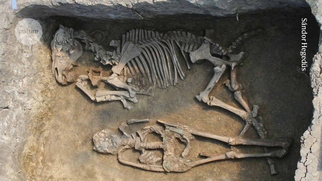
  • Ancient DNA traces family lines and political shifts in the Avar empire

    Ancient DNA traces family lines and political shifts in the Avar empire

    [ad_1]

    Nature, Published online: 24 April 2024; doi:10.1038/d41586-024-01020-9

    Genetic pedigrees spanning nine generations uncover the social organization of a nomadic empire that dominated much of central and eastern Europe from the sixth to the early ninth century.

    [ad_2]

    Source link

  • Charles Darwin investigates: the curious case of primrose punishment

    Charles Darwin investigates: the curious case of primrose punishment

    [ad_1]

    Nature, Published online: 23 April 2024; doi:10.1038/d41586-024-01180-8

    Birds emerge as top suspects for unexplained flower mutilation, and reflections from 1974 mark the 21st anniversary of the discovery of the DNA double helix, in the weekly dip into Nature’s archive.

    [ad_2]

    Source link

  • A step along the path towards AlphaFold — 50 years ago

    A step along the path towards AlphaFold — 50 years ago

    [ad_1]

    Nature, Published online: 16 April 2024; doi:10.1038/d41586-024-01094-5

    Paring down the astronomical complexity of the protein-folding problem, plus Isaac Newton’s ambiguous use of the word ‘axiom’, in the weekly dip into Nature’s archive.

    [ad_2]

    Source link

  • The biologist who built a Faraday cage for a crab

    The biologist who built a Faraday cage for a crab

    [ad_1]

    Nature, Published online: 09 April 2024; doi:10.1038/d41586-024-00919-7

    What every biologist should know about electronics, plus a disturbing outbreak of volcanism in North Carolina, in the weekly dip into Nature’s archive.

    [ad_2]

    Source link

  • understanding the horror of genocide

    understanding the horror of genocide

    [ad_1]

    Thousands of people gather at the Kicukiro College of Technology football pitch to commemorate the 2,000 people who were abandoned by United Nations troops during the 1994 genocide April 5, 2014 in Kigali, Rwanda.

    Much of the research on the genocide against Tutsi communities has neglected the testimonies of survivors.Credit: Chip Somodevilla/Getty

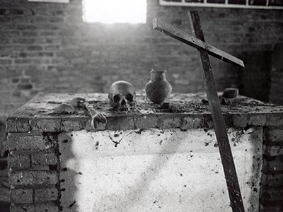
    This month marks 30 years since the start of the 1994 genocide against Rwanda’s Tutsi communities. Around 800,000 Tutsi were killed by armed Hutu militia and citizens over 100 days. Members of the Hutu and Twa communities also died, in what some scholars call the worst atrocity of the late twentieth century.

    This 30th anniversary is a poignant reminder of many things, but perhaps first and foremost of the international community’s failure to intervene and stop the killings. Massacres of Tutsi people had been happening for decades before 1994, but calls for help from inside Rwanda were ignored, with horrific consequences.

    This week, in a News Feature commemorating the anniversary of the atrocity, Nature has spoken to researchers about what has been learnt about the genocide, the consequences for its survivors and its aftermath. Lessons from studying a specific genocide can be applicable to many events that involve conflict.

    The 1948 Convention on the Prevention and Punishment of the Crime of Genocide, adopted after the Second World War, defines genocide as “an act committed with intent to destroy, in whole or in part, a national, ethnical, racial or religious group”. It is, the convention states, an “odious scourge” that “at all periods of history … has inflicted great losses on humanity”.

    Genocide is incredibly difficult to study. The hardest question of all concerns a genocide’s origins: how wars and violence can escalate to genocidal acts. At the same time, genocide studies is not one discipline. It spans the political and social sciences, anthropology, biology, economics, history, law, medicine, sociology and more. Researchers bring individual disciplinary insights, but must also collaborate. Nature heard from researchers studying peace-building between communities affected by the genocide, and learnt about mental-health approaches that have helped survivors. We also spoke to scientists who have studied how the trauma from the event has marked the DNA of survivors and their children. Intergenerational trauma — trauma relating to the genocide that affects younger generations who did not directly experience it — remains a challenge for mental-health services in Rwanda. But this is a legacy of all atrocities, and one that societies should be prepared for.

    In Rwanda’s case, the genocide nearly wiped out the country’s academic community; until recently, the study of the atrocity had largely been done by researchers from other countries. Rwanda’s scholars have re-established themselves and must be supported so they can lead the study of genocide, political violence and beyond. The country already hosts some of Africa’s notable research institutions, including a chapter of the African Institute for Mathematical Sciences in Kigali and the African Medicines Agency, soon to be established in the capital.

    Researchers in African countries face many barriers. They consistently report that international journals are too quick to reject their submissions. Some told Nature that this might be because of a perception that research from low-income nations or countries with limited academic autonomy is of low quality. One exceptional effort that is helping to overcome these barriers is the Research, Policy and Higher Education programme, focused on Rwanda. Now a decade old and launched by the UK-based charity Aegis Trust in Nottingham, this programme invites Rwandan scholars to submit research proposals; external researchers support them with advice and expertise to get the works published in international venues, such as peer-reviewed journals. The resulting works are collected in a resource called the Genocide Research Hub.

    So far, more than 40 scholars have published dozens of journal articles, book chapters and working papers. Some studies have already influenced Rwandan policy relating to the genocide. For example, Rwandan scholar Munyurangabo Benda, a philosopher of religion at the Queen’s Foundation, an ecumenical college in Birmingham, UK, investigated feelings of guilt among children of Hutu perpetrators born after the genocide. A peace-building project that involved this generation of children grew into a nationwide programme on reconciliation. Benda’s academic research played a part in broadening the programme’s offerings.

    In the immediate aftermath of atrocities, focus is often put on perpetrators, as legal organizations seek to make convictions and secure justice. But, in the study of genocide, it is imperative to listen to survivors, to establish their needs and how they can be supported, and also to ensure that their testimonies and experiences are not lost.

    Much of the research on the genocide against the Tutsi has neglected the testimonies of survivors, particularly women, says Noam Schimmel, a scholar of international studies and human rights at the University of California, Berkeley. Survivors need to be given opportunities to share and write about their own perspectives and experiences — whether in literature, as part of research or in journalism — which can help to overcome isolation and marginalization, and to improve their well-being and welfare.

    As atrocities continue to unfold around the world, researchers can learn from Rwanda. Those in positions of responsibility must allow researchers from affected countries to lead where they can, and to elevate the voices of survivors. In doing so, they will bring a deeper level of experience that might allow us to better study and understand these heinous acts. We might still be far from answers — but greater knowledge can only help to shine more light on this darkest of places.

    [ad_2]

    Source link

  • The Internet Archive Just Backed Up an Entire Caribbean Island

    The Internet Archive Just Backed Up an Entire Caribbean Island

    [ad_1]

    Aruba’s colonial history also meant documents were spread all over the place. “Our collection was scattered,” says Edric Croes, the head of archival conservation and management at the National Archives of Aruba. There were works to be scanned across the world, including in the Netherlands, Spain, the United States, and other islands like Curaçao. Establishing a hub to find the documents online has been especially helpful, Scholing notes, for researchers located abroad, who no longer have to travel to Aruba to physically dig through archives.

    It’s unusual for a country to outsource this sort of project to a foreign nonprofit. “In a dream world, every national library would have enough funds to bring on an amazing team of people,” says University of Waterloo history professor Ian Milligan, who is writing a book on the Internet Archive’s origins, and was not involved in the Aruba project. “Governments often don’t have that.”

    The Internet Archive has not previously acted as custodian of a country’s whole collection, although it has worked with a number of national and regional libraries around the world. Back in 2011, it partnered with the Culture Office of Bali, an island province of Indonesia, to preserve what the office described at the time as “90 percent of Bali’s literature.” (This now makes up the Internet Archive’s Balinese Digital Library collection.)

    Aruba’s archivists hope other nations will follow in its digital footsteps. “It’s a really feasible model that could be applied to a lot of small islands, developing states, even bigger countries with limited means,” Scholing says.

    Partnering with the Internet Archive looks like an obvious solution for cash-strapped archivists. Potential partners do need to think, though, about what it means to rely on another country’s private organization, one with its own challenges.

    “When we think about digital preservation, we often think of the technical challenges,” says Milligan of Waterloo. “But I think the biggest challenges are the social challenges, the human challenges. How can you set up an organization that will be here in 50 years?”

    He credits the Internet Archive with a very “sustainable structure,” in terms of future-proofing. But that doesn’t make it wholly invulnerable. The Archive is currently facing a number of serious legal challenges, including a lawsuit from major record labels, including Universal Music Group, Capitol, and Sony, that poses an existential threat—the labels are asking for damages that could amount to over $400 million.

    That’s on top of an ongoing dispute with publishing companies over a digital lending library it established during the pandemic. While its digitization capabilities are far more robust than many nation-states, the Internet Archive’s position in an increasingly vituperative battleground between copyright holders and tech companies means that its future is precarious, too.

    The Internet Archive sees Aruba’s endorsement as especially timely. “It’s been really empowering to see that the nation of Aruba is continuing to add materials and upload content at the same time that we’re facing this,” Freeland says. “We’re in this for the long haul.”

    [ad_2]

    Source link