LBCC dataset and processing
The original LBCC dataset included 123,984 MRI scans from 101,457 human participants across more than 100 studies (which include multiple publicly available datasets46,47,48,49,50,51,52,53,54,55,56) and was described in previous work4 (see Supplementary Information and supplementary table S1 from ref. 4). We filtered to the subset of cognitively normal participants whose data were processed using FreeSurfer (v6.1). Studies were curated for the analysis by excluding duplicated observations and studies with fewer than 4 unique age points, sample size less than 20 and/or only participants of one sex. If there were fewer than three participants having longitudinal observations, only the baseline observations were included and the study was considered cross-sectional. If a participant had changing demographic information during the longitudinal follow-up (for example, changing biological sex), only the most recent observation was included. We updated the LBCC dataset with the ABCD release 5, resulting in a final dataset that includes 77,695 MRI scans from 60,900 cognitively normal participants with available total GMV, sGMV and GMV measures across 63 studies (Supplementary Table 1). In this dataset, 74,148 MRI scans from 57,538 participants across 43 studies have complete-case regional brain measures (regional GMV, regional surface area and regional cortical thickness, based on Desikan–Killiany parcellation20; Supplementary Table 2). The global brain measure mean cortical thickness was derived using the regional brain measures (see below).
Structural brain measures
Details of data processing have been described in our previous work4. In brief, total GMV, sGMV and WMV were estimated from T1-weighted and T2-weighted (when available) MRIs using the ‘aseg’ output from FreeSurfer (v6.0.1). All three cerebrum tissue volumes were extracted from the aseg.stats files output by the recon-all process: ‘Total cortical gray matter volume’ for GMV; ‘Total cerebral white matter volume’ for WMV; and ‘Subcortical gray matter volume’ for sGMV (inclusive of the thalamus, caudate nucleus, putamen, pallidum, hippocampus, amygdala and nucleus accumbens area; https://freesurfer.net/fswiki/SubcorticalSegmentation). Regional GMV and cortical thickness across 68 regions (34 per hemisphere, based on Desikan–Killiany parcellation20) were obtained from the aparc.stats files output by the recon-all process. Mean cortical thickness across the whole brain is the weighted average of the regional cortical thickness weighted by the corresponding regional surface areas.
Preprocessing specific to ABCD
Functional connectivity measures
Longitudinal functional connectivity measures were obtained from the ABCD-BIDS community collection, which houses a community-shared and continually updated ABCD neuroimaging dataset available under Brain Imaging Data Structure (BIDS) standards. The data used in these analyses were processed using the abcd-hcp-pipeline (v0.1.3), an updated version of The Human Connectome Project MRI pipeline57. In brief, resting-state functional MRI time series were demeaned and detrended, and a generalized linear model was used to regress out mean white matter, cerebrospinal fluid and global signal, as well as motion variables and then band-pass filtered. High-motion frames (filtered frame displacement > 0.2 mm) were censored during the demeaning and detrending. After preprocessing, the time series were parcellated using the 352 regions of the Gordon atlas (including 19 subcortical structures) and pairwise Pearson correlations were computed among the regions. Functional connectivity measures were estimated from resting-state fMRI time series using a minimum of 5 min of data. After Fisher’s z-transformation, the connectivities were averaged across the 24 canonical functional networks25, forming 276 inter-network connectivities and 24 intra-network connectivities.
Cognitive and other covariates
The ABCD dataset is a large-scale repository aiming to track the brain and psychological development of over 10,000 children 9–16 years of age by measuring hundreds of variables, including demographic, physical, cognitive and mental health variables58. We used release 5 of the ABCD study to examine the effect of the sampling schemes on other types of covariates including cognition (fully corrected T-scores of the individual subscales and total composite scores of the NIH Toolbox24), mental health (total problem CBCL syndrome scale) and other common demographic variables (BMI, birth weight and handedness). For each of the covariates, we evaluated the effect of the sampling schemes on their associations with the global and regional structural brain measures and functional connectivity after controlling for non-linear age and sex (and for functional connectivity outcomes only, mean frame displacement).
For the analyses of structural brain measures, there were three non-brain covariates with fewer than 5% non-missing follow-ups at both 2-year and 4-year follow-ups (that is, the Dimensional Change Card Sort Test, Cognition Fluid Composite and Cognition Total Composite Score; Supplementary Table 11), and only their baseline cognitive measurements were included in the analyses. For the remaining 11 variables (that is, the Picture Vocabulary Test, Flanker Inhibitory Control and Attention Test, List Sorting Working Memory Test, Pattern Comparison Processing Speed Test, Picture Sequence Memory Test, Oral Reading Recognition Test, Crystallized Composite, CBCL, birth weight, BMI and handedness), all of the available baseline, 2-year and 4-year follow-up observations were used. For the analyses of the functional connectivity, only the baseline observations for the List Sorting Working Memory Test were used due to missingness (Supplementary Table 12).
The records with BMI lying outside the lower and upper 1% quantiles (that is, BMI < 13.5 or BMI > 36.9) were considered misinput and replaced with missing values. The variable handedness was imputed using the last observation carried forwards.
Statistical analysis
Removal of site effects
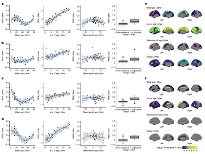
For multisite or multistudy neuroimaging studies, it is necessary to control for potential heterogeneity between sites to obtain unconfounded and generalizable results. Before estimating the main effects of age and sex on the global and regional brain measures (total GMV, total WMV, total sGMV, mean cortical thickness, regional GMV and regional cortical thickness), we applied ComBat21 and LongComBat22 in cross-sectional datasets and longitudinal datasets, respectively, to remove the potential site effects. The ComBat algorithm involves several steps including data standardization, site-effect estimation, empirical Bayesian adjustment, removing estimated site effects and data rescaling.
In the analysis of cross-sectional datasets, the models for ComBat were specified as a linear regression model illustrated below using total GMV:
$${\rm{GMV\; \sim \; ns(age,\; d.f.\; =\; 2)\; +\; sex\; +\; site}},$$
where ns denotes natural cubic splines on 2 d.f., which means that there were two boundary knots and one interval knot placed at the median of the covariate age. Splines were used to accommodate non-linearity in the age effect. For the longitudinal datasets, the model for LongComBat used a linear mixed effects model with participant-specific random intercepts:
$${\rm{GMV\; \sim \; (1| participant)\; +\; ns(age,\; d.f.\; =\; 2)\; +\; sex\; +\; site}}.$$
When estimating the effects of other non-brain covariates in the ABCD dataset, ComBat was used to control the site effects, respectively, for each of the cross-sectional covariates. The ComBat models were specified as illustrated below using GMV:
$${\rm{GMV\; \sim \; ns(age,\; d.f.\; =\; 2)\; +\; sex}}+x+{\rm{site,}}$$
where x denotes the non-brain covariate. LongComBat was used for each of the longitudinal covariates with a linear mixed effects model with participant-specific random intercepts only:
$${\rm{GMV\; \sim \; (1| participant)\; +\; ns(age,\; d.f.\; =\; 2)\; +\; sex}}+x+{\rm{site.}}$$
When estimating the effects of other covariates on the functional connectivity (FC) in the ABCD data, we additionally controlled for the mean frame displacement (FD) of the frames remaining after scrubbing. The longComBat models were specified as:
$$\begin{array}{l}\text{FC}\, \sim \,(1| \text{participant})+\text{ns}(\text{age, d.f.}=2)\,+\,\text{sex}\\ \,+\,\text{ns}(\text{mean}\_\text{FD, d. f.}=3+x+\text{site}.\end{array}$$
The Combat and LongComBat were implemented using the neuroCombat59 and longCombat60 R packages. Site effects were removed before all subsequent analyses including the bootstrap analyses described below.
RESI for association strength
The RESI is a recently developed standardized effect size index that has consistent interpretation across many model types, encompassing all types of test statistics in most regression models17,18. In brief, the RESI is a standardized effect size parameter describing the deviation of the true parameter value (or values) \(\beta \) from the reference value (or values) \({\beta }_{0}\) from the statistical null hypothesis \({H}_{0}:\,\beta ={\beta }_{0}\),
$$S=\sqrt{{(\beta -{\beta }_{0})}^{T}{{\varSigma }_{\beta }}^{-1}(\beta -{\beta }_{0})},$$
where S denotes the parameter RESI, \(\beta \) and \({\beta }_{0}\) can be vectors, T denotes the transpose of a matrix, \({\varSigma }_{\beta }\) is the covariance matrix for \(\sqrt{N}\hat{\beta }\) (where \(\hat{\beta }\) is the estimator for \(\beta \), N is the number of participants; section 3 in Supplementary Information).
In previous work, we defined a consistent estimator for RESI17,
$$\hat{S}={\left(\max \left\{0,\frac{{T}^{2}-m}{N}\right\}\right)}^{1/2},$$
where \({{T}}^{2}\) is the chi-squared test statistics \({T}^{2}=N{(\beta -{\beta }_{0})}^{T}{{\varSigma }_{\beta }}^{-1}(\beta -{\beta }_{0})\) for testing the null hypothesis \({H}_{0}:\,\beta ={\beta }_{0}\), \(m\) is the number of parameters being tested (that is, the length of \(\beta \)) and \(N\) is the number of participants.
As RESI is generally applicable across different models and data types, it is also applicable to the situation where Cohen’s d was defined. In this scenario, the RESI is equal to ½ Cohen’s d17, so Cohen’s suggested thresholds for effect size can be adopted for RESI: small (RESI = 0.1), medium (RESI = 0.25) and large (RESI = 0.4). Because RESI is robust, when the assumptions of Cohen’s d are not satisfied, such as when the variances between the groups are not equal, RESI is still a consistent estimator, but Cohen’s d is not. The confidence intervals for RESI in our analyses were constructed using 1,000 non-parametric bootstraps18.
The systematic difference in the standardized effect sizes between cross-sectional and longitudinal studies puts extra challenges on the comparison and aggregation of standardized effect size estimates across studies with different designs. To improve the comparability of standardized effect sizes between cross-sectional and longitudinal studies, we proposed a new effect size index: the cross-sectional RESI (CS-RESI) for longitudinal datasets. The CS-RESI for longitudinal datasets represents the RESI in the same study population if the longitudinal study had been conducted cross-sectionally. Detailed definition, point estimator and confidence interval construction procedure for CS-RESI can be found in section 3 in Supplementary Information. Comprehensive statistical simulation studies were also performed to demonstrate the valid performance of the proposed estimator and confidence interval for CS-RESI (section 3.2 in Supplementary Information). With CS-RESI, we can quantify the benefit of using a longitudinal study design in a single dataset (section 3.3 in Supplementary Information).
Study-level models
After removing the site effects using ComBat or LongComBat in the multisite data, we estimated the effects of age and sex on each of the global or regional brain measures using GEEs and linear regression models in the longitudinal datasets and cross-sectional datasets, respectively. The mean model was specified as below after ComBat or LongComBat:
$${y}_{ij} \sim {\rm{ns}}({{\rm{age}}}_{ij},{\rm{d.f.}}=2)+{{\rm{sex}}}_{i},$$
where yij was taken to be a global brain measure (that is, total GMV, WMV, sGMV or mean cortical thickness) or regional brain measure (that is, regional GMV or cortical thickness) at the j-th visit from the participant i and j = 1 for cross-sectional datasets. The age effect was estimated with natural cubic splines with 2 d.f., which means that there were two boundary knots and one interval knot placed at the median of the covariate age. For the GEEs, we used an exchangeable correlation structure as the working structure and identity linkage function. The model assumes the mean was correctly specified, but made no assumption about the error distribution. The GEEs were fitted with the ‘geepack’ package61 in R. We used the RESI as a standardized effect size measure. RESIs and confidence intervals were computed using the ‘RESI’ R package (v1.2.0)19.
Meta-analysis of the age and sex effects
The weighted linear regression model for the meta-analysis of age effects across the studies was specified as:
$${\widehat{S}}_{{\rm{age}},k}={{\rm{design}}}_{k}+{\rm{ns}}[{\rm{mean}}{({\rm{age}})}_{k},3]+{\rm{ns}}[{\rm{s.d.}}{({\rm{age}})}_{k},3]+{\rm{ns}}[{\rm{skew}}{({\rm{age}})}_{k},3]+{{\epsilon }}_{k},$$
where \({\widehat{S}}_{{\rm{age}},k}\) denotes the estimated RESI for study k, and the weights were the inverse of the standard error of each RESI estimate. The sample mean, standard deviation (s.d.) and skewness of the age were included as non-linear terms estimated using natural splines with 3 d.f. (that is, two boundary knots plus two interval knots at the 33rd and 66th percentiles of the covariates), and a binary variable indicating the design type (cross-sectional or longitudinal) was also included.
The weighted linear regression model for the meta-analysis of sex effects across the studies was specified as
$${\widehat{S}}_{{\rm{sex}},k}={{\rm{design}}}_{k}+{\rm{ns}}[{\rm{mean}}{({\rm{age}})}_{k},3]+{\rm{ns}}[{\rm{s.d.}}{({\rm{age}})}_{k},3]+{\rm{ns}}[{\rm{pr}}{({\rm{male}})}_{k},3]+{{\epsilon }}_{k},$$
where \({\widehat{S}}_{{\rm{sex}},k}\) denotes the estimated RESI of sex for study k, and the weights were the inverse of the standard error of each RESI estimate. The sample mean, standard deviation of the age covariate and the proportion of males in each study were included as non-linear terms estimated using natural splines with 3 d.f., and a binary variable indicating the design type (cross-sectional or longitudinal) was also included.
These meta-analyses were performed for each of the global and regional brain measures. Inferences were performed using robust standard errors62. In the partial regression plots, the expected standardized effect sizes for the age effects were estimated from the meta-analysis model after fixing mean age at 45 years, standard deviation of age at 7 years and/or skewness at 0; the expected standardized effect sizes for the sex effects were estimated from the meta-analysis model after fixing mean age at 45 years, standard deviation of age at 7 years and/or proportion of males at 0.5.
Sampling schemes for age in the UKB and ADNI
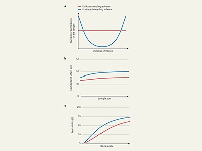
We used bootstrapping to evaluate the effect of different sampling schemes with different target sample covariate distributions on the standardized effect sizes and replicability in the cross-sectional UKB and longitudinal ADNI datasets. For a given sample size and sampling schemes, 1,000 bootstrap replicates were conducted. The standardized effect size was estimated as the mean standardized effect size (that is, RESI) across the bootstrap replicates. The 95% confidence interval for the standardized effect size was estimated using the lower and upper 2.5% quantiles across the 1,000 estimates of the standardized effect size in the bootstrap replicates. Power was calculated as the proportion of bootstrap replicates producing P values less than or equal to 5% for those associations that were significant at 0.05 in the full sample. In the UKB, only one region was not significant for age in each of GMV and cortical thickness, and in the ADNI, only one and four regions were not significant for age in GMV and cortical thickness, respectively. Replicability in previous work has been defined as having a significant P value and the same sign for the regression coefficient. Because we were fitting non-linear effects, we defined replicability as the probability that two independent studies have significant P values; this is equivalent to the definition of power squared. The 95% confidence intervals for replicability were derived using Wilson’s method63.
In the UKB dataset, to modify the (between-subject) variability of the age variable, we used the following three target sampling distributions (Extended Data Fig. 1a): bell shaped, where the target distribution had most of the participants distributed in the middle age range; uniform, where the target distribution had participants equally distributed across the age range; and U shaped, where the target distribution had most of the participants distributed closer to the range limits of the age in the study. The samples with U-shaped age distribution had the largest sample variance of age, followed by the samples with uniform age distribution and the samples with bell-shaped age distribution. The bell-shaped and U-shaped functions were proportional to a quadratic function. To sample according to these distributions, each record was first inversely weighted by the frequency of the records with age falling in the range of ±0.5 years of the age for that record to achieve the uniform sampling distribution. Each record was then rescaled to derive the weights for bell-shaped and U-shaped sampling distributions. The records with age < 50 or age > 78 years were winsorized at 50 or 78 years when assigning weights, respectively, to limit the effects of outliers on the weight assignment, but the actual age values were used when analysing each bootstrapped data.
In each bootstrap from the ADNI dataset, each participant was sampled to have two records. We modified the between-subject and within-subject variability of age, respectively, by making the ‘baseline age’ follow one of the three target sampling distributions used for the UKB dataset and the ‘age change’ independently follow one of three new distributions: decreasing, uniform and increasing (Extended Data Fig. 1b,c). The increasing and decreasing functions were proportional to an exponential function. The samples with increasing distribution of age change had the largest within-subject variability of age, followed by the samples with the uniform distribution of age change and the samples with decreasing distribution of age change.
To modify the baseline age and the age change from baseline independently, we first created all combinations of the baseline record and one follow-up from each participant, and derived the baseline age and age change for each combination. The ‘bivariate’ frequency of each combination was obtained as the number of combinations with values of baseline age and age change falling in the range of ±0.5 years of the values of baseline age and age change for this combination. Then, each combination was inversely weighted by its bivariate frequency to target a uniform bivariate distribution of baseline age and age change. The weight for each combination was then rescaled to make the baseline age and age change follow different sampling distributions independently. The combinations with baseline age < 65 or age > 85 years were winsorized at 65 or 85 years, and the combinations with age change greater than 5 years were winsorized at 5 years when assigning weights to limit the effects of outliers on the weight assignment, but the actual ages were used when analysing each bootstrapped data.
The sampling methods could be easily extended to the scenario in which each participant had three records (and more than three) in the bootstrap data by making combinations of the baseline and two follow-ups. Each combination was inversely weighted to achieve uniform baseline age and age change distributions, respectively, by the ‘trivariate’ frequency of the combinations with baseline age and the two age changes from baseline for the two follow-ups falling into the range of ±0.5 years of the corresponding values for this combination. As we only investigated the effect of modifying the number of measurements per participant under uniform between-subject and within-subject sampling schemes (Fig. 3c,d), we did not need to consider rescaling the weights here to achieve other sampling distributions but they could be done similarly. For the scenario in which each participant only had one measurement (Fig. 3c,d), the standardized effect sizes and replicability were estimated only using the baseline measurements.
All site effects were removed using ComBat or LongComBat before performing the bootstrap analysis.
Sampling schemes for other non-brain covariates in the ABCD
We used bootstrapping to study how different sampling strategies affect the RESI in the ABCD dataset. Each participant in the bootstrap data had two measurements. We applied the same weight assignment method described above for the ADNI dataset to modify the between-subject and within-subject variability of a covariate. We made the baseline covariate and the change in covariate follow bell-shaped and/or U-shaped distributions, to let the sample have larger or smaller between-subject and/or within-subject variability of the covariate, respectively. The baseline covariate and change of covariate were winsorized at the upper and lower 5% quantiles to limit the effect of outliers on sampling. For each cognitive variable, only the participants with non-missing baseline measurements and at least one non-missing follow-up were included.
Generalized linear models and GEEs were fitted to estimate the effect of each non-brain covariate on the structural brain measures after controlling for age and sex,
$${\rm{GMV}} \sim {\rm{ns}}({\rm{age,\; d.f.}}=2)+{\rm{sex}}+x,$$
where x denotes one of the non-brain covariates. For the GEEs, we used an exchangeable correlation structure as the working structure and identity linkage function.
Only the between-subject sampling schemes were applied for the non-brain covariates that were stable over time (for example, birth weight and handedness). In other words, the participants were sampled based on their baseline covariate values, and then a follow-up was selected randomly for each participant. The sampling schemes to increase the between-subject variability in the covariate handedness, which was a binary variable (right-handed or not), was specified differently. The expected proportion of right-handed participants in the bootstrap samples was 50% under the sampling scheme with larger between-subject variability and 10% under the sampling scheme with smaller between-subject variability.
For given between-subject and/or within-subject sampling schemes, we obtained 1,000 bootstrap replicates. The standardized effect size was estimated as the mean standardized effect size across the bootstrap replicates. The 95% confidence intervals for standardized effect size were estimated using the lower and upper 2.5% quantiles across the 1,000 estimates of the standardized effect size in the bootstrap replicates. The sample sizes needed for 80% replicability were estimated based on the (mean) estimated standardized effect size and F-distribution (see below).
Analysis of functional connectivity in the ABCD
In a subset of the ABCD in which we have preprocessed longitudinal functional connectivity data at two time points (baseline and 2-year follow-up), we only restricted our analysis to the participants with non-missing measurements at both of the two time points. In the GEEs used to estimate the effects of non-brain covariates on functional connectivity, the mean model was specified as below after LongComBat:
$${y}_{ij} \sim {\rm{ns}}({{\rm{age}}}_{ij},{\rm{d.f.}}=2)+{{\rm{sex}}}_{i}+{\rm{ns}}({\rm{mean}}\_{\rm{FD}},\mathrm{d.f.}=3)+x,$$
where yij was taken to be a functional connectivity outcome, and x denotes a non-brain covariate. The mean frame-wise displacement (mean_FD) was also included as a covariate with natural cubic splines with 3 d.f. We used an exchangeable correlation structure as the working structure and identity linkage function in the GEEs. The frame count of each scan was used as the weights.
When evaluating the effect of different sampling schemes on the standardized effect sizes, we obtained 1,000 bootstrap replicates for given between-subject and/or within-subject sampling schemes. The standardized effect size was estimated as the mean standardized effect size across the bootstrap replicates. Confidence intervals were computed as described above. The sample sizes needed for 80% replicability were estimated based on the (mean) estimated standardized effect sizes and F-distribution (see below).
Sample size calculation for a target power or replicability with a given standardized effect size
After estimating the standardized effect size for an association, the calculation of the corresponding sample size N needed for detecting this association with γ × 100% power at significance level of α was based on an F-distribution. d.f. denotes the total degree of freedom of the analysis model, \(F(z;\lambda )\) denotes the cumulative density function for a random variable z, which follows the (non-central) F-distribution with degrees of freedom being 1 and N − d.f. and non-centrality parameter \(\lambda \). The corresponding sample size N is:
$$N=\{N:F({F}^{-1}(1-\alpha )\,;\lambda =N{\hat{S}}^{2})=\gamma \},$$
where \(\hat{S}\) is the estimated RESI for the standardized effect size. Power curves for the RESI are given in figure 3 of Vandekar et al.17. Replicability was defined as the probability that two independent studies have significant P values, which is equivalent to power squared.
Estimation of the between-subject and within-subject effects
For the non-brain covariates that were analysed longitudinally in the ABCD dataset, GEEs with exchangeable correlation structures were fitted to estimate their cross-sectional and longitudinal effects on structural and functional brain measures after controlling for age and sex, respectively. The mean model was specified as illustrated with GMV:
$${\rm{GMV\; \sim \; ns(age,\; d.f.\; =\; 2)\; +\; sex}}+X\_{\rm{bl}}+X\_{\rm{change,}}$$
where X_bl denotes the participant-specific baseline covariate values, and the X_change denotes the difference of the covariate value at each visit to the participant-specific baseline covariate value (see section 5.2 in Supplementary Information). The participants without baseline measures were not included in the modelling. The model coefficients for the terms X_bl and X_change represent the between-subject and within-subject effects of this non-brain covariate on total GMV, respectively. For the functional connectivity data, the same covariates and weighting were used as described above. Using the first time point as the between-subject term was a special case that ensured that comparing the parameter using the baseline cross-sectional model was equal to the parameter for the between-subject effect in the longitudinal model. In this model, the between-subject variance was defined as the variance of the baseline measurement, and the within-subject variance was the mean square of X_change. This model specification ensured that the sampling schemes independently affected the between-subject and within-subject variances separately (equation (16) in section 5.2 in Supplementary Information).
Reporting summary
Further information on research design is available in the Nature Portfolio Reporting Summary linked to this article.