



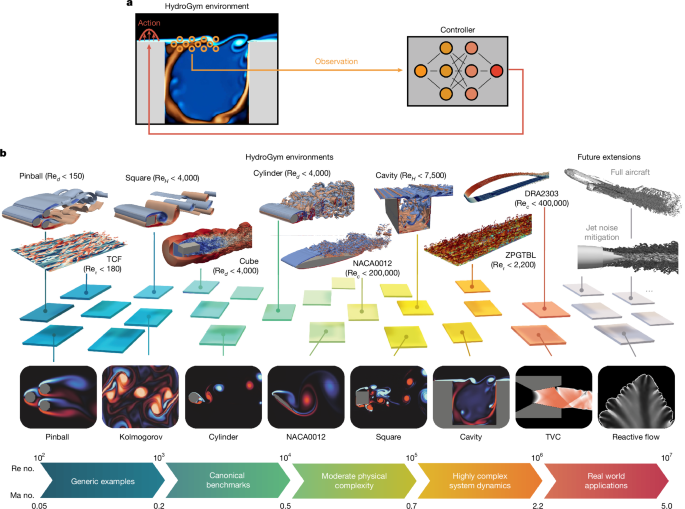
The HydroGym platform formulates flow control problems as discrete-time Markov decision processes, defined by the tuple \(({\mathcal{S}},{\mathcal{A}},{\mathcal{P}},{\mathcal{R}})\). At each control step t, the agent: receives an observation state \({s}_{t}\in {\mathcal{S}}\), which represents flow measurements; executes an action \({a}_{t}\in {\mathcal{A}}\), which represents actuator inputs; and receives a scalar reward \({r}_{t}\in {\mathcal{R}}\) that quantifies the control objective (for example, drag reduction or flow stabilization). The transition probability \({\mathcal{P}}\) is governed implicitly by the underlying Navier–Stokes equations integrated by the fluid solver.
To bridge the gap between machine learning and fluid dynamics, HydroGym uses the Farama Foundation Gymnasium interface44, abstracting the complexity of the CFD execution. This abstraction is illustrated by the straightforward initialization and interaction pattern for an open cavity control example:
# Swap one line to switch backend solvers
import hydrogym.firedrake as hgym
# import hydrogym.maia as hgym
# import hydrogym.nek as hgym
# import hydrogym.jax as hgym
# import hydrogym.jaxfluids as hgym
# initialize environment
env = hgym.FlowEnv(‘Cavity_2D_Re7500’, **kwargs)
# reset environment
obs, info = env.reset()
# interact with environment
for i in range(num_interactions):
obs, reward, terminated, truncated, info = env.step(action)
This design enables control and machine learning engineers to focus on algorithmic development without CFD expertise, while providing fluids researchers access to state-of-the-art RL techniques. The solver-independent architecture ensures that advances in CFD can be seamlessly integrated into the platform without disrupting existing workflows.
A critical element of the Markov decision processes formulation in HydroGym is the temporal coupling between the physical solver and the RL agent. As turbulent flows evolve continuously while RL agents typically assume discrete actions, control inputs are updated at fixed intervals Δtctrl, which correspond to multiple physical CFD time steps designed to capture the characteristic timescale of the target instabilities (for example, vortex shedding or shear-layer oscillation).
To prevent numerical instabilities arising from discontinuous boundary conditions, HydroGym enforces temporal smoothing on all control actions. The instantaneous actuation magnitude A(t) is smoothly interpolated between the previous action Aold and the new target action Anew over a predefined number of sub-iterations using a hyperbolic tangent or exponential ramp function. Furthermore, to standardize learning across disparate physical regimes, all observation features and action bounds are inherently normalized to the [−1, 1] range within the environment wrapper.
Computational fluid dynamics backends
To accommodate diverse computational scales ranging from rapid prototyping to large-scale high-performance computing (HPC) campaigns, HydroGym implements a solver-independent architecture supporting multiple backends. All computational environments have been thoroughly validated against established benchmarks to ensure physical correctness and high-fidelity resolution of the underlying fluid dynamics. Comprehensive validation studies and grid convergence analyses for each solver and flow configuration are detailed in Supplementary Sections 3 and 5.
Lattice Boltzmann solver (m-AIA LB)
For the majority of weakly compressible, large-scale two- and three-dimensional DNS, HydroGym uses the lattice Boltzmann method embedded within the m-AIA solver framework45, which has been continuously developed at RWTH Aachen University for over two decades. The solver evolves the discrete particle distribution function fi on a D3Q27 velocity lattice via a two-step collision–streaming update. At low-to-moderate Reynolds numbers, a Bhatnagar–Gross–Krook (BGK) collision operator is used, relaxing distributions towards a local Maxwellian equilibrium with a single relaxation frequency ωBGK linked to the kinematic viscosity. To enhance stability at higher Reynolds numbers, a cumulant-based collision operator is used instead, performing relaxations in a cumulant space with individual rates ωα (ref. 46). Local grid refinement follows the methodology proposed by Eitel-Amor and colleagues47, adjusting ωBGK across hierarchical grid levels to preserve a constant kinematic viscosity throughout the domain. No-slip boundaries are represented via a second-order interpolated bounce-back scheme. A hybrid parallelization strategy built on the message passing interface (MPI) and a shared memory model either based on open multi-processing (OpenMP) or on the parallel algorithms in the C++ standard provided by the NVIDIA HPC SDK and AMD ROCm HIPSTDPAR backends allows for a hardware-agnostic GPU implementation.
Finite-volume solver (m-AIA FV)
Beyond the lattice Boltzmann method, m-AIA includes a compressible Navier–Stokes solver based on a finite-volume method targeting DNS and large-eddy simulation (LES) of wall-bounded turbulent flows at higher Mach numbers. The compressible Navier–Stokes equations are cast in an arbitrary Lagrangian–Eulerian formulation and discretized on structured, body-conforming curvilinear grids with a cell-centred scheme, which enables anisotropic mesh refinement in the wall-normal direction suited for flat-plate and airfoil configurations. Inviscid fluxes are evaluated with the advection upstream splitting method combined with Monotonic Upstream-centred Scheme for Conservation Laws reconstruction for second-order spatial accuracy, whereas viscous fluxes are discretized using a modified cell-vertex approach. Temporal integration uses a five-stage, low-storage Runge–Kutta scheme; when the grid deforms under surface actuation, the geometric conservation law is enforced at every stage. Subgrid-scale effects in under-resolved LES are handled implicitly via a monotonically integrated LES strategy, exploiting the inherent numerical dissipation of the upwind-biased advection upstream splitting method scheme. The finite-volume code shares the same MPI/OpenMP/GPU parallelization strategy as the lattice Boltzmann solver. For RL integration, the solver exposes both synthetic jet actuation and a travelling transversal surface-wave boundary condition14,48,49,50,51, where the wave amplitude A, wavelength λ, and phase speed c serve as time-varying control parameters updated by the agent at each control step via a C1-continuous cosine cross-fade transition to ensure numerical stability.
Spectral-element solver (Nek5000)
For incompressible high-Reynolds-number configurations requiring higher-order accuracy, HydroGym provides a Nek500052 backend using the spectral-element method. The velocity and pressure fields are approximated by high-order Lagrange interpolants on hexahedral elements following the \({{\mathbb{P}}}_{N}{{\mathbb{P}}}_{N-2}\) formulation53: velocity is collocated onto N3 Gauss–Lobatto–Legendre points per element, whereas pressure resides on a staggered grid of (N − 2)3 Gauss–Legendre points. Temporal integration combines a third-order explicit extrapolation scheme for the nonlinear convective terms with a third-order implicit backward differentiation scheme for viscous contributions. Aliasing errors are mitigated by overintegration, with an oversampling factor of 3/2 in each spatial direction. Flow actuation is prescribed as a time-dependent wall-normal Dirichlet velocity vn with the spatial mean removed to satisfy the ZNMF constraint. Parallelization is achieved through a hybrid OpenMPI distributed- and shared-memory strategy, and coupling with RL agents is implemented via dynamic MPI-based communication.
Differentiable incompressible solver
To enable gradient-enhanced reinforcement learning28, HydroGym provides natively differentiable solvers written in JAX54 for the incompressible Navier–Stokes equations. The Kolmogorov flow environment uses a pseudo-spectral method with two-thirds de-aliasing on a doubly periodic domain, advancing the vorticity–streamfunction formulation with a fourth-order Runge–Kutta scheme. The three-dimensional turbulent channel flow uses a fully differentiable finite-difference DNS solver, in which spatial derivatives are formed with sparse differentiation matrices, and the pressure Poisson equation is solved via a biconjugate gradient-stabilized method. Both environments implement a Gymnax interface55 and inherit RL frameworks from PureJaxRL56, enabling a fully synchronous training pipeline compatible with JAX’s automatic differentiation. Exact analytical gradients of the objective with respect to control parameters are obtained via jax.grad through the entire simulation trajectory. Parallelization across multiple random seeds is achieved using vmap for batch processing, and just-in-time compilation via jit optimizes execution on GPU hardware.
Differentiable compressible solver (JAX-Fluids)
For gradient-based flow control in compressible and multiphase regimes, HydroGym integrates the JAX-Fluids solver57,58—a fully-differentiable, high-order CFD code written entirely in Python using the JAX library. The compressible Navier–Stokes equations are solved on structured Cartesian grids, with arbitrary one-dimensional mesh stretching. Convective fluxes are evaluated using either fifth-order weighted essentially non-oscillatory (WENO5-Z), or sixth-order targeted essentially non-oscillatory (TENO6-A) shock-capturing reconstruction, coupled with an approximate Harten–Lax–van Leer–Contact Riemann solver. Diffusive fluxes are evaluated using high-order central differences, and time integration is performed with explicit total variation diminishing Runge–Kutta schemes. Multiphase flows are supported through both a sharp-interface level-set method and a five-equation diffuse-interface model. Positivity-preserving limiters are used to ensure robust integration in the presence of strong shocks or large density ratios. The level-set implementation in JAX-Fluids further functions as an immersed boundary method, enabling flow simulations around complex geometries. The immersed boundary method is particularly well suited for active flow control problems, as control actions (for example, blowing or suction) can be naturally incorporated through interface exchange terms. By adhering strictly to JAX’s functional programming model, the entire simulation pipeline is end-to-end differentiable. Exact gradients of arbitrary scalar objectives, for example, time-averaged drag or RL reward, with respect to control inputs or neural network weights are backpropagated through the full temporal trajectory via jax.grad or value_and_grad, with gradient checkpointing (jax.checkpoint) mitigating memory overhead for long rollouts. For large-scale HPC deployment, JAX-Fluids uses homogeneous domain decomposition across multiple accelerated linear algebra devices via jax.pmap, with inter-block halo exchanges performed exclusively through jax.lax.ppermute to keep the automatic differentiation graph intact across distributed, multi-node clusters.
Finite-element solver (Firedrake)
For maximum code transparency and rapid prototyping of two-dimensional control problems, HydroGym provides a Firedrake59 backend built on the Portable, Extensible Toolkit for Scientific Computation, which offers automatic code generation for variational problems. The incompressible Navier–Stokes equations are discretized with Taylor–Hood elements (second-order continuous Galerkin for velocity, first-order for pressure) to ensure inf–sup stability, and time integration uses fully implicit schemes, with an automatic solver-parameter selection based on the Reynolds number and grid resolution. The implementation follows a three-tier modular architecture separating the physical problem definition (PDEBase), time-stepping (TransientSolver) and RL interfacing (FlowEnv), with the last module implementing the Farama Foundation Gymnasium interface and translating between RL concepts and CFD operations. Parallelization leverages Firedrake’s distributed mesh capabilities and the Portable, Extensible Toolkit for Scientific Computation’s parallel sparse linear algebra routines.
Reinforcement learning and multi-agent infrastructure
Rather than heavily tuning hyperparameters for each configuration, which would hinder generalizability, HydroGym relies on robust observation and action normalization to ensure standard off-the-shelf RL algorithms serve as strong baselines. The platform integrates seamlessly with StableBaselines360, TorchRL61 and CleanRL62 for model-free continuous control, and PureJaxRL for natively differentiable environments. For standard model-free environments, we evaluated PPO, DDPG and TD3.
Gradient-enhanced PPO
HydroGym implements GPPO for differentiable environments. Standard PPO relies on likelihood ratio methods or generalized advantage estimation to estimate policy gradients. In GPPO, the analytical gradient of the reward trajectory with respect to the policy parameters, \({\nabla }_{\theta }{{\mathbb{E}}}_{\tau \sim {\pi }_{\theta }}[\sum R({s}_{t},{a}_{t})]\) is computed exactly by backpropagating through the deterministic fluid dynamics solver. This analytical gradient is incorporated into PPO’s clipped surrogate objective, drastically reducing variance and improving sample efficiency.
Multi-agent reinforcement learning
HydroGym implements a decentralized MARL architecture to tackle the dimensionality barrier of spatially distributed 3D flows (such as 3D cylinders, channel and airfoil flows). Global control domains are partitioned into locally invariant pseudo-environments. Multiple agents operate on these local partitions and may share a common control policy π(a∣s). To ensure unbiased data distributions in the shared replay buffer, overlapping mesh nodes are excluded from the pseudo-environment definitions, whereas identical actuation is enforced at boundary interfaces to preserve control continuity. Communication between the parallelized CFD domains and the centralized RL policy is managed efficiently via an MPI-based interface.
Further details regarding the reinforcement learning agents are provided in Supplementary Section 4.
Environment set-up for discussed results
Although the configurations discussed in the main text are briefly outlined below, comprehensive details concerning the physical characteristics, exact boundary conditions, observation or action space normalizations, and specific reward formulations for all environments are provided in Supplementary Section 5.
Circular cylinder (Re = 3,900)
The subcritical 3D cylinder flow represents a highly chaotic wake. The computational domains extend [51.2D × 48D] in 2D and 32D × 16D × 4D with periodic spanwise boundaries in 3D. Actuation is applied via ZNMF synthetic jets positioned at the top and bottom of the cylinder. The reward function targets drag minimization while penalizing lift oscillations: r = −∣CD∣ − ω∣CL∣. For MARL configurations, the span is decomposed into independent pseudo-environments, each controlling local jet pairs.
Fluidic pinball (Re = 100−150)
The pinball environment features three circular cylinders in an equilateral triangle layout, exposing agents to multiple bifurcation regimes, including symmetry-breaking pitchfork bifurcations and chaotic dynamics. The control mechanism consists of the independent surface rotation of all three cylinders. The reward formulation targets collective drag reduction: \(r=-{\sum }_{i=1}^{3}| {C}_{D,i}| \,-\) \(\omega {\sum }_{i=1}^{3}| {C}_{L,i}| \), where the scaling factor ω restricts policies from exploiting asymmetric lift generation.
Open cavity flow (Re = 4,200−7,500)
The cavity flow targets the stabilization of complex feedback loops and Kelvin–Helmholtz instabilities at the shear layer spanning the cavity opening. The reward function penalizes deviations of observed flow quantities from a target reference state: \(r=-{\sum }_{i}{\left(\frac{{{\rm{obs}}}_{i}-{\bar{o}}_{i}}{{{\sigma }}_{i}}\right)}^{2}\), where obsi represents pressure and velocity measurements at shear-layer probes, \({\bar{o}}_{i}\) is the target mean approximated over 1,000 instability cycles and σi provides normalization scaling. Actuation is performed using localized jet actuators at the upstream cavity edge and, optionally, inside the cavity, providing multi-point flow manipulation to disrupt resonant interactions.
Transverse gust mitigation (NACA0012, Re = 1,000)
This environment simulates extreme aerodynamic conditions using a highly disturbed inflow. A 1-cosine transverse gust with a gust ratio G = 2.0 interacts with an airfoil at a high angle of attack (α = 20°), threatening dynamic stall and severe load fluctuations. Control is achieved via three independent jet actuators distributed along the leading edge, each covering 3% of the chord length. The reward function is designed to minimize gust-induced force variance while preserving the baseline aerodynamic efficiency: \(r=-| {C}_{L}(t)-{\bar{C}}_{L,\mathrm{ref}}| -\omega | {C}_{D}(t)-{\bar{C}}_{D,\mathrm{ref}}| \).
Physics-guided transfer learning and zero-shot deployment
HydroGym uses a physics-guided zero-shot transfer protocol to bridge the gap between computationally tractable RL training and prohibitive industrial-scale CFD. This method was used to control the suction-side turbulent boundary layer (TBL) of a NACA0012 wing section at a chord-based Reynolds number of Rec = 200,000.
Surrogate construction and pre-training
Direct RL exploration on the high-resolution wing is computationally prohibitive. Instead, our working hypothesis argues that the target control region on the wing (ranging from x/c = 0.25 to 0.86) can be systematically partitioned into smaller chordwise blocks based on the local Clauser pressure-gradient parameter β, with a surrogate environment constructed for each. For the symmetric NACA0012 configuration at a 0° angle of attack evaluated here, the moderate adverse pressure gradient across the control region naturally yields a single, continuous control block. Consequently, a single surrogate turbulent channel flow (TCF) is generated. Furthermore, the near-wall spatial resolution of the TCF matches the wing simulations in viscous units (Δx+, Δy+, Δz+), ensuring that the effective footprint of the controllers remains geometrically consistent.
Agents are trained exclusively within these TCF surrogates using the MARL framework (TD3 algorithm). The observation space relies strictly on near-wall metrics accessible in real-world scenarios: the wall-tangential (\(u{\prime} \)) and wall-normal (\(v{\prime} \)) velocity fluctuations sampled at a sensing plane of y+ = 15. The action a dictates the wall-normal blowing or suction velocity, strictly bounded by the local friction velocity (−uτ ≤ a ≤ uτ) and subjected to a ZNMF constraint across the control region. The reward function seeks to minimize the relative wall-shear stress, \(r=1-{\tau }_{w}^{\mathrm{ctrl}}/{\tau }_{w}^{\mathrm{ref}}\).
Zero-shot deployment
Following training in the idealized TCF surrogates, the optimized policies are deployed directly onto the corresponding partitioned blocks of the 3D NACA0012 wing sections. No further on-wing training or fine-tuning is performed. To map the policies appropriately, the agent’s observations are standardized using the spatially varying viscous scales of the wing. As the viscous time unit t* evolves along the wing chord, the update frequency of the deployed actions is scaled by the local streamwise-averaged friction velocity \({\langle {u}_{\tau }\rangle }_{x}\) of each respective block. By learning generalized responses to near-wall streaks rather than overfitting to the macroscopic geometry of the channel, the RL policies successfully attenuate high-speed streaks on the wing, yielding substantial reductions in skin-friction drag at a fraction of the computational cost (~104 magnitude reduction in required core-hours compared to direct on-wing training). Baseline comparison methods include uniform blowing and opposition control63.