


Ethics statement
All experiments involving human cell lines were approved by the Harvard University IRB and ESCRO committees. All animal experiments were conducted according to protocols approved by the Institutional Animal Care and Use Committee (IACUC) of Harvard University. All experiments were performed in accordance with relevant guidelines and regulations, and in accordance with informed consent obtained from the donors of the originating cells or tissues.
Mouse experiments and housing
To develop the mouse-endogenous chimeroid system, we used wild-type CD-1 and C57BL/6 mice (Charles River Laboratories). We used embryos of both sexes, collected at E11.5. The sex of each embryo was not determined prior to the experiment. Sample size was not predetermined using specific methods. Mice were maintained under standard housing conditions in a temperature- and humidity-controlled facility under a 12 h–12 h light–dark cycle (light, 07:00 to 19:00) with ad libitum access to food and water. The ambient temperature was maintained at 20–24 °C and the relative humidity at 30–70%.
Human pluripotent stem cell culture
All human PS cell lines were maintained as previously detailed7,9. In brief, MTESR1 medium (StemCell Technologies), mTESR+ medium (StemCell Technologies) or StemFlex medium (Gibco), all with 1% of added penicillin–streptomycin Solution (Corning), were employed for culture of stem cells in cell culture dishes (Falcon) precoated with 1% Geltrex (Gibco), at 37 °C in 5% CO2. All human PS cells were maintained below passage 55 and tested negative for mycoplasma (assayed using the MycoAlert PLUS Mycoplasma Detection Kit, Lonza).
Characterization of the PS cell lines
The psychiatric control Mito210 male iPS cell line was provided by B. Cohen (McLean Hospital); the PGP1 male iPS cell line was provided by G. Church; the GM08330 male iPS cell line was provided by M. Talkowski (MGH) and was originally derived from fibroblasts obtained from the Coriell Institute for Medical Research6,7,30. The H1 male human embryonic stem cell line (also known as WA01) was purchased from WiCell; and the 11a iPS cell line was obtained from the Harvard Stem Cell Institute. The female CW50037 iPS cell line was from the California Institute for Regenerative Medicine (CIRM) iPS cell collection. All lines were authenticated as follows. The PGP1 iPS cell line was authenticated by short-tandem-repeat (STR) analysis (performed by TRIPath). The 11a cell line was authenticated by karyotyping as previously described40. The Mito210 iPS cell line was authenticated with genotyping analysis (Fluidigm FPV5 chip) performed by the Broad Institute Genomics Platform. The CW50037 iPS cell line was authenticated using single-nucleotide polymorphism (SNP) genotyping (Illumina Global Screening Array (GSA) from Illumina; processed at the Genomics Platform, Broad Institute) for cell line identification and detection of chromosomal abnormalities. The H1 and GM08330 lines were authenticated by STR analysis (performed by WiCell). The GM08330 parental line has a previously reported30 interstitial duplication in the long (q) arm of chromosome 20; all other lines were karyotypically normal. No commonly misidentified lines were used in this study.
Cortical organoid and chimeroid differentiation
Dorsally patterned cortical organoids were generated following a protocol previously published by our group7. In brief, on day 0, feeder-free cultured human PS cells, 75–85% confluent, were enzymatically dissociated to single cells with Accutase (Gibco), and 9,000 cells per well were reaggregated in ultra-low-cell-adhesion 96-well plates with V-bottom conical wells (sBio PrimeSurface plate; Sumitomo Bakelite) using the same pluripotent cell medium in which they were previously maintained. At day 1, 80 μl of medium was replaced with cortical differentiation medium (CDM) I, containing Glasgow-MEM (Gibco), 20% knockout serum replacement (Gibco), 0.1 mM minimum essential medium non-essential amino acids (MEM-NEAA) (Gibco), 1 mM pyruvate (Gibco), 0.1 mM 2-mercaptoethanol (Gibco), with 1% of penicillin–streptomycin solution (Corning). From day 0 to day 6, ROCK inhibitor Y-27632 (Millipore) was added to the medium at a final concentration of 20 μM. Patterning small molecules, WNT inhibitor IWR1 (Calbiochem) and TGFβ inhibitor SB431542 (Stem Cell Technologies), were added from day 0 to day 18, at a concentration of 3 μM and 5 μM, respectively.
Single-donor and multidonor chimeroids were generated as previously described9. In brief, patterned EBs between day 15–18 were dissociated into single-cell suspensions using a modified papain-based protocol9. After confirming morphology, organoids were enzymatically and mechanically dissociated, then filtered and resuspended in CDM1 medium with ROCK inhibitor. Cell suspensions from different donors (in the case of multidonor chimeroids) were mixed in equal ratios and reaggregated (18,000–20,000 cells per well) in ultra-low-adhesion 96-well plates. Then, 2 days later, embryoid bodies were transferred to low-attachment dishes and cultured under orbital agitation. Medium was sequentially changed to CDM2, CDM3 (at DIV35) and CDM4 (at DIV70) as per established protocols7. For APM, organoids at day 70 were transferred into a medium containing BrainPhys Basal (Stem Cell Technologies), 20 ng ml−1 N2 supplement (1×, Thermo Fisher Scientific), 20 ng ml−1 B27 supplement (1×, Thermo Fisher Scientific), 1% penicillin–streptomycin solution 100× (Corning), 1% MEM-NEAA (Gibco), 1% GlutaMax (Gibco) and amphotericin B (Thermo Fischer Scientific). After filtration, GDNF and BDNF at a final concentration of 20 ng ml−1 were added. Along with dCAMP (MilliporeSigma), ascorbic acid (StemCell Technologies) and laminin (Thermo Fischer Scientific) at a concentration of 1 mM, 200 nM and 1 μg ml−1. Half of the medium was replaced with fresh medium twice per week. Heterochronic and monochronic cultures were obtained using the previously described chimeroid strategy; however, papain dissociation time and mechanical dissociation were adjusted based on organoid age (25 min for younger organoids; for older organoids, mincing with a blade followed by 45 min of digestion). While the chimeroid strategy is extremely efficient in younger organoids, the success rate of the heterochronic cultures remains very low. This is probably due to the dual requirement for sufficient patterning in the young organoids and adequate stemness in the older cells, both of which are necessary to ensure robust signalling from the young tissue and sufficient recovery of older cells for analysis at day 14 after mixing. Chimeroids derived from old organoids were smaller than those derived from young organoids, probably due to the limited proliferative potential of the old neural progenitors. Organoid time-series include at least n = 6 organoids/3 batches at all stages (6 months to 5 years).
Mouse experiments
We used wild-type CD1 and C57BL/6 mice (Charles River Laboratories). Pregnant dams were euthanized to obtain embryos. Embryos were staged carefully according to Theiler stages for E11.5 and the neocortex was dissected. Stage-matched embryos were pooled (15–20 per experiment) prior to dissociation. The dissociation protocol described for the human chimeroids was used with some modifications. Dissociated progenitors were seeded to aggregate overnight at a density of 12,000 cells per well. The next day, the medium was switched to CDM2 for 3 days. On day 4 after seeding, the medium was changed to CDM3 and then to CDM4 on day 6. We quantified the number of nuclei with positive SATB2 expression across three condition groups: monochronic (old), monochronic (young) and heterochronic from cultures 1 day (D1AM; for each group: n = 3 replicate organoids × 3 batches) and 2.5 days (D2.5AM; for each group: n = 3 replicate organoids × 1 batch) after mixing, respectively. For evaluating the overall effect of condition on the proportion of nuclei with positive SABT2 expression at D1AM, binomial generalized linear models (GLMs) were used to model the number of SATB2-positive nuclei out of total nuclei per organoid and adjust for batch by including batch as a fixed effect. Models with or without adding a condition as a fixed effect were evaluated by a likelihood ratio test using the anova function. Following the observation of the global effect of the condition being statistically significant (ANOVA, P < 0.05), estimated marginal means for each group were derived from the fitted full binomial GLM by using the R package emmeans, and Tukey-adjusted pairwise comparisons were performed between groups. For D2.5AM, due to the absence of more than one batch level to adjust for, we proceeded with computing estimated marginal means and performing pairwise comparisons between groups.
To fluorescently label neurons, we incubated cells while aggregating with AAV particles encoding GFP under the CAG promoter. The AAV serotype PHPeB permits efficient transduction of the central nervous system36. Organoids were fixed and imaged around 3weeks after aggregation on the LSM900 microscope. Images were acquired using the Zeiss microscope and processed in ImageJ (v.2.14.0/1.54 f). pAAV-CAG-GFP was acquired from Addgene (Addgene, 37825).
Statistical analysis
Organoids used for analysis or treatment were chosen from each batch to be representative of the morphology seen in that differentiation. For every experiment, organoids were collected without a preconceived selection strategy or priority. The investigators did not use blinding in this study. However, our analytical pipeline for each experiment followed uniform criteria applied to all samples, allowing us to analyse our data in an unbiased manner. All bioinformatics analyses were applied uniformly to all samples without considering genotype adjustments. Sample size was not predetermined using specific methods. At least three organoids were used for each experiment, guided by analysis from previous published work6,7,30. This prior research demonstrated the reproducibility of this organoid system and confirmed that using three organoids adequately captured variation.
Fixation and processing of samples for cryosectioning
Organoids were fixed in 4% paraformaldehyde (PFA) (Electron Microscopy Services) overnight in a 12-well plate (Falcon) at 4 °C, washed three times with 1× PBS (Gibco), and cryoprotected in a 30% sucrose solution (Sigma-Aldrich) in PBS overnight at 4 °C.
Gelatin solution containing 10% bovine gelatin (Sigma-Aldrich) and 7.5% sucrose (Sigma-Aldrich) was prewarmed at 37 °C for 15 min. The 30% sucrose solution was removed from the samples and exchanged for the prewarmed gelatin, and the samples were incubated at 37 °C for 15 min. Meanwhile, plastic moulds were coated with a 2 mm layer of warm gelatin solution and left to polymerize at room temperature. The samples were then transferred to the pretreated plastic moulds, and 1 ml of warm gelatin solution was added on top. After polymerization at room temperature for 3 min, the samples were prechilled at 4 °C for 15–20 min. Finally, the moulds were frozen in a cold bath containing 100% ethanol and dry ice for 2–3 min, and stored at −80 °C indefinitely.
Immunohistochemistry
For immunohistochemistry, 14–18 μm-thick sections were cut using the cryostat (Leica). Cryosections were stabilized at room temperature for 5 min and blocked with 10% donkey serum (Sigma-Aldrich) + 0.3% Triton X-100 (Sigma-Aldrich) in PBS. Primary antibodies (Supplementary Table 15) were diluted in the blocking solution and incubated overnight. After four washes with PBS, cryosections were incubated at room temperature with secondary antibodies diluted in PBS (1:1,000; Supplementary Table 15) for 1 h at room temperature, washed four times with PBS and stained with DAPI (1:10,000 in PBS + 0.1% Tween-20) for 5 min to visualize cell nuclei. At later timepoints (>1 year), we consistently observed a reduction in staining specificity, with increased background signal that limited reliable interpretation of most antibodies, despite extensive optimization. For the 2–3 year organoid immunohistochemistry, we used the fresh-frozen protocol described below.
Immunohistochemistry on fresh-frozen sections
Human brain organoids aged 2 to 5.8 years were rinsed with PBS, directly embedded in OCT compound (NEG-50, Richard-Allen Scientific) and then quickly frozen. Fresh-frozen OCT blocks were cryosectioned at 10 µm thickness. The sections were thawed onto Superfrost Plus Gold glass slides (EMS). Organoid depths of 0–150 μm were collected as serial sections. Sections were fixed in ice-cold methanol at −20 °C for 20 min, then rinsed with PBST0.1 (1× PBS with 0.1% Tween-20). Permeabilization was performed with PBST0.25 (1× PBS with 0.25% Tween-20) for 15 min. Blocking was done with 5% donkey or goat serum in PBST0.5 (1× PBS with 0.5% Tween-20) for 30 min. Alexa-Fluor-conjugated antibodies (NEUN/RBFOX3; 608455, BioLegend) were diluted 1:200 in blocking buffer and incubated with sections for 1–2 h. The sections were rinsed with PBST0.1 and incubated with 0.2 μg ml−1 DAPI for 3 min, then rinsed with PBS and water. ProLong Gold anti-fade mounting medium was applied, and coverslips were mounted. Images were acquired using LSM900 with Zeiss software. Image processing was done using ImageJ (v.2.14.0/1.54f). NeuN-positive nuclei were observed up to approximately 80 μm deep, beyond which they were not observed.
Hypoxyprobe assay
Hypoxyprobe (pimonidazole HCl; Hypoxyprobe Kit HPI-100) was applied to n = 3 1-year-old CDM4 organoids at a final concentration of 100 µM. Organoids were incubated with the probe for 1.5 h at 37 °C and 5% CO2. Samples were then washed with PBS, fixed in 4% PFA at room temperature for 2 h, embedded and sectioned at 14 µm. Immunohistochemistry was performed according to the manufacturer’s instructions, and the primary antibody included in the kit was used at a 1:50 dilution6.
Whole-organoid immunofluorescence
Organoids were washed in wash buffer (PBS with 0.4% BSA) and fixed at room temperature for 30 min with 4% PFA. After fixation, organoids were stored in 1× PBS with 0.1% Tween-20 (P9416, Sigma-Aldrich). Permeabilization, blocking and staining were performed as previously described41. Nuclei were counterstained with 0.5 μg ml−1 DAPI for 30 min. Organoids were optically cleared using RIMS and mounted as previously described41,42. Images were acquired with LSM880 (Zeiss) and LSM900 (Zeiss) using a ×40 objective. Images were processed with ImageJ (v.2.14.0/1.54f). Nuclei were segmented and quantified using ZEN blue v.3.1 Image Analysis and Intellesis software packages. Image segmentation was achieved using a previously trained ZEN Intellesis algorithm43. SATB2 intensity was thresholded to define positive nuclei and counted across the various z-stacks of individual organoids.
Microscopy
Immunofluorescence images were acquired using the Zeiss Axio Imager.Z2 with a ×20 objective (pixel size, 0.325 μm) using the Apotome optical sectioning function. The Zen Blue software was used to perform tile stitching and apotome deconvolution before exporting the images. For the LSM900, z stacks with 3 μm step size were acquired with a ×20 objective (pixel size, 0.62 μm), followed by tile stitching using the Zen Blue software. Further processing, such as z projections, channel merging and adding scale bars, was performed in Fiji v.43. Images were adjusted for brightness and contrast; all adjustments were applied to the whole image.
SATB2 and FOS quantification
Nine-month-old organoids from three genetic backgrounds (H1, PGP1 and 11a) were analysed (n = 3 organoids per condition per line; APM and CDM4). Three regions per organoid were randomly selected based on DAPI signal and imaged from three sections on the same slide. z-Stacks were acquired using a 20× objective (0.62 µm per pixel; 3 µm step size; 3–5 optical sections) on a Zeiss system (Zen Blue). Acquisition settings were as follows: SATB2 (650 V, 2%, 28 µm pinhole), FOS (750 V, 10%, 31 µm) and DAPI (650 V, 1%, 27 µm). Stacks were converted to average-intensity projections and quantified in Fiji (v.43). SATB2-positive cells were defined as DAPI-positive nuclei with elevated SATB2 signal and were subsequently assessed for FOS expression.
Bulk RNA-seq from organoids
Snap-frozen organoids were resuspended in RLT buffer containing β-mercaptoethanol, and RNA was isolated with a DNase digestion step according to the manufacturer’s protocol (RNeasy, Qiagen). Then, 10 ng of RNA was used for library preparation with the Smart-Seq Pico input total RNA library preparation kit, including ZapR depletion (with unique molecular identifiers (UMIs)), according to the recommended protocol. Libraries were quantified, pooled and sequenced on the NextSeq 2000 (Illumina) instrument.
DNA extraction and methylome analyses
Genomic DNA extraction and WGBS
Genomic DNA was isolated from organoids using a previously described method44. In brief, organoids were thawed on ice and suspended in 500 μl of resuspension buffer (240 μl of genomic lysis buffer (D4075, Zymo), 20 μl of proteinase K (D4075, Zymo) and 240 μl of nuclease-free water). The sample was thoroughly mixed, vortexed and incubated at 55 °C for 4 to 7 h at 300 rpm. An equal volume of phenol:chloroform:isoamyl alcohol (15593031, Thermo Fisher Scientific) was added, mixed by inversion and then centrifuged at 13,000g for 5 min. The aqueous phase (around 400 μl) was transferred to a new tube for precipitation. To this aqueous phase, 8 μl of Glycogen-Blue (AM9515, Thermo Fisher Scientific), 20 μl of 5 M NaCl (AM9760G, Thermo Fisher Scientific) and 1 ml of ethanol (E7023, Sigma-Aldrich) were added, mixed by inversion, and allowed to precipitate overnight at −20 °C. The tubes were spun at 13,000g for 45 min at 4 °C. The supernatant was discarded and 1 ml of 70% ethanol was added to the pellet, which was then spun down at 13,000g for 45 min at 4 °C. The supernatant was discarded, and the pellet was air-dried for 10 min before being resuspended in elution buffer (low-EDTA TE pH 8, 15575020, Thermo Fisher Scientific) and incubated at 55 °C for 10 min.
Genomic DNA was fragmented in a tube (MicroTube AFA Fiber pre-slit snap-cap 6 × 16 mm, 520045, Covaris) using a Covaris S-series S2 Sonicator with the following settings: duty cycle, 10%; intensity, 5; cycles per burst, 200; maximum temperature, 7 °C; duration, 76–90 s. Fragmented DNA was purified and concentrated using the DNA Clean & Concentrator kit (D4013, Zymo) and eluted in 22 µl of low TE (pH 8). 1 µl of the eluate was used for quality control on the Agilent TapeStation (HSD5000), resulting in an average fragment size of 237–322 bp. Bisulfite conversion was performed using the EZ DNA Methylation-Gold kit (D5005, Zymo), with the final converted DNA eluted in 16 µl of low TE (pH 8). Libraries were prepared using the xGen-Methyl-Seq DNA Library prep kit (10009824, IDT), in combination with xGen UDI Primer Plate 2 (8 nucleotides, 10009816, IDT). The number of PCR cycles used was 7. Each library underwent two final rounds of purification using AMPure XP beads (A63881, Beckman Coulter). Libraries were assessed for concentration, fragment size distribution and primer-dimer absence using the Agilent TapeStation (HSD5000). Sequencing was conducted on the Illumina NovaSeq 6000 and Element Biosciences Aviti platform, generating 150 base paired-end reads, targeting 800–900 million reads per sample.
WGBS processing
Raw reads were subjected to adapter and quality trimming using cutadapt45 (v.4.6; parameters: –quality-cutoff 20 –overlap 5 –minimum-length 25; Illumina TruSeq adapter clipped from both reads), followed by trimming of 10 and 5 nucleotides from the 5′ and 3′ end of the first read and 15 and 5 nucleotides from the 5′ and 3′ end of the second read. Trimmed reads were aligned to the human reference genome (hg19) using BSMAP46 (v.2.90; parameters: -v 0.1 -s 16 -q 20 -w 100 -S 1 -u -R). In this study, we used hg19 (rather than the current hg38) as the reference genome to maintain compatibility and coordinate consistency with previously generated reference datasets, annotation resources and downstream comparative analyses incorporated into our methylation analysis pipeline, including publicly available developmental brain methylation datasets and established epigenetic clock resources. Importantly, all samples and comparative analyses were processed uniformly within the same reference framework. Because our analyses focused primarily on genome-wide and regional DNA methylation patterns rather than fine-resolution structural variation or novel genomic annotations, we do not expect the use of hg19 versus hg38 to materially affect the biological conclusions of the study. Sorted BAM files were generated and indexed using samtools47 with the ‘sort’ and ‘index’ commands (v.1.21). Duplicates were removed using the MarkDuplicates command from GATK (v.4.5.0.0; –VALIDATION_STRINGENCY = LENIENT –REMOVE_DUPLICATES=true –COMPRESSION_LEVEL 4 –ASSUME_SORT_ORDER coordinate)48. Methylation rates were called using mcall from the MOABS49 package (v.1.3.9.6; default parameters; –reportCpX A/C/T for non-CpG methylation calling). All methylation analyses were restricted to autosomes and only CpGs covered by at least 10 and at most 150 reads were considered for downstream analyses. Assessment of global, genome-wide methylation was performed using average (arithmetic mean) methylation levels. Region-specific methylation was assessed by calculating average methylation levels across features (bins, partially methylated domains, highly methylated domains, DMVs, repeats, cdDMRs, superenhancers) using bigWigAverageOverBed from UCSC tools for each sample, where a feature was only considered if at least three CpGs were contained measurements within a region.
Endogenous comparison
cdDMRs defined from postnatal human brain were obtained from ref. 14. cdDMR coordinates in hg19 and their cluster assignment based on cell-type-specific methylation trajectories (six clusters: 1:G−N+, 2:G0N+, 3:G0N−, 4:G+N0, 5:G+N−, 6:G−N0) were used as provided by the study. cdDMRs were scored for mean methylation in organoid samples using bigWigAverageOverBed as described above (≥3 CpGs covered). To quantify recapitulation of temporal methylation dynamics in organoids, for each cdDMR, a linear regression model was fitted predicting mean cdDMR methylation from time in culture (in months), yielding a slope estimate (change in methylation per month). cdDMRs were classified as showing temporal changes over time in organoids if the absolute slope value had a minimum of 0.1/60 (corresponding to a predicted minimum change of 0.1 in methylation rate over 60 months). The fetal brain DNAm age was estimated using the FetalClock function from ref. 18, based on the implementation provided at GitHub (https://github.com/LSteg/EpigeneticFetalClock).
Differential methylation analysis
DMRs were called using metilene50 (v.0.2-8). DMRs were defined by an absolute minimum difference in methylation of 0.1 with a maximum distance of 300 nucleotides between CpGs within a DMR and a minimum of 10 CpGs per DMR and Bonferroni correction for multiple testing (parameters: –m 10 –c 1 –d 0.1) and filtered by q < 0.05. DMRs were classified as hypo-DMRs and hyper-DMRs based on the direction of change. DMRs were associated with CGIs and DMVs based on a minimum overlap of 1 bp. DMRs were annotated to the nearest genes using GREAT51 (v.4.0.4; default parameters).
To identify temporal changes in methylation, DMRs were called between early and late culture timepoints (3 months versus 5 years). DMRs were filtered to retain only those with a minimum absolute Pearson correlation coefficient of 0.6 between time in culture (in months) and mean DMR methylation rate across all timepoints.
To evaluate effects of APM on the methylation landscape, DMRs were called between organoids cultured for 9 months or 1 year in CDM4 and organoids cultured for 9 months or 1 year in APM.
Genomic feature annotation
CGIs were obtained from the UCSC Genome Browser (https://genome-euro.ucsc.edu/cgi-bin/hgTables). CpG shores were defined as 2 kb regions flanking CGIs upstream and downstream; shelves were defined as 2 kb regions flanking the shores.
DMVs were defined based on WGBS data from the HUES64 human embryonic stem cell line52. To identify DMVs, a previously described sliding-window approach was adapted53. In brief, 5 kb windows with a 1 kb step size were generated across autosomes using bedtools54 makewindows. Average CpG methylation was calculated for each window, excluding CpGs located within CGIs, and separately for CGIs. Windows and CGIs with an average methylation below 0.15 and containing at least 10 CpGs were merged, excluding regions composed solely of CGIs.
Annotations of highly methylated domains and partially methylated domains were obtained from GitHub (https://zwdzwd.github.io/pmd)55.
Repeat annotations were obtained from the hg19 UCSC RepeatMasker track, excluding entries on alternative haplotypes, fix patches and chrMT.
Epigenetic clocks
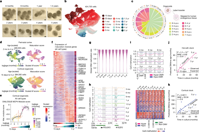
CpG methylation values at low-coverage sites (coverage < 5) were imputed using the boostme package (v.0.1.0). Imputation was performed on individual samples represented as objects from the bsseq package (v.1.40.0). Imputed values exceeding one were capped at one. Array-based probe IDs were mapped to genomic coordinates using the Illumina EPIC array manifest (EPIC.hg19.manifest). The pan-tissue human methylation clock17 was applied using the DNAmAge function from the methylclock56 package (v.1.10.0). Cortical DNA methylation age57 was estimated using the CorticalClock function based on the implementation provided at GitHub (https://github.com/gemmashireby/CorticalClock). DNAm age was assessed by the median absolute error between the time in culture of the organoids and the predicted methylation age in months, as well as Pearson correlation between the two across all samples.
To assess mitotic history, DNA methylation at solo-WCGW CpGs, which are particularly susceptible to methylation loss with cell division55, was quantified. Methylation was evaluated across three feature sets: all solo-WCGWs, solo-WCGWs within common PMDs and solo-WCGWs in common PMDs represented on the HM450 array. Annotations were obtained from https://zwdzwd.github.io/pmd, and the average methylation levels across feature sets were calculated per sample from non-imputed WGBS data.
mCA
Forebrain superenhancers were obtained from a previously published dataset of fetal human brain tissue and cerebral organoids15. The mean mCA levels at these regions were compared with the background levels calculated across genome-wide 30 kb bins (approximating the average superenhancer size), excluding bins overlapping with superenhancers.
Locus methylation trend plots
For regions of interest (ROIs), the mean methylation was computed using bigWigAverageOverBed as described above (≥3 CpGs covered) and modelled as a function of time in culture (in months) using linear regression. Trends were visualized using per-ROI scatterplots with fitted regression lines (and 95% confidence intervals) and Pearson correlation estimates.
Visualizations
Unless stated otherwise, all statistics and plots were generated using R v.4.4.1. Violin plots were generated using the vioplot (v.0.5.1) or ggplot2 (v.3.5.2) package and show the kernel density estimation with embedded box plots indicating the median, interquartile range and whiskers extending to 1.5× the interquartile range. Circos plots were created using the RCircos (v.1.2.2) package from tracks with averaged profiles over 50 kb bins created using UCSC tools bigwigAverageOverBed. The differential signal was obtained by subtracting the 5-year profile from the 3-month profile. Cytoband and ideogram data for hg19 were obtained from the RCircos package. DMR methylation heat maps and average tracks were created using the EnrichedHeatmap58 package (v.1.34.0) by applying the normalizeToMatrix function first, with 2,500 bp extensions up- and downstream and a target ratio of 0.4. Pairwise genome-wide correlations of methylation rates between samples of consecutive timepoints were plotted using the smoothScatter function. The box plots show the median (centre line), interquartile range (box) and the whiskers extend to 1.5× the interquartile range; individual observations are overlaid as points. Bar plots, box plots, scatter plots and line plots were created using ggplot2.
Electrophysiological analyses
Electrical signals were recorded using the Accura 3D CMOS-HD-MEA system by 3Brain (BioCAM DupleX system, in combination with Accura 3D chips). The 3D chip contains 4,096 penetrating µNeedle electrodes with 90 µm height arranged in 64 × 64 grid in a square measuring 3.8 × 3.8 mm, with a sampling rate of 20 kHz and a 12-bit resolution. CDM4 organoids were changed to APM medium 14–21 days before recording, and acute recordings from intact organoids were performed at 37 °C in a mini-incubator box filled with Carbogen. BrainWave v.5 was used to record spontaneous activity for 15–20 min. To test whether the electrical activity measured was synaptic, NMDA and AMPA receptor activity was blocked at the end of recordings using D-AP5 (150 μM) and DNQX (30 μM), respectively. Moreover, action potentials were blocked by bath application of TTX (1 μM). Spike detection was carried out by Kilosort231, followed by analysis of the spike train using custom MATLAB scripts (v.24.1, R2024b, The MathWorks). The detection of rapid spiking periods (burst) was performed by implementing the maximum interval59 algorithm (maximum interval = 170 ms, maximum end interval = 400 ms, minimum interval between bursts = 800 ms, minimum duration of burst = 40 ms, minimum number of spikes = 4). The analysis of network bursting was performed on the basis of the population-averaged spiking rate along all detected units. A peak in the population signal was considered to be a network burst if it met the following criteria: (1) the peak amplitude was greater than 4× the s.d. of the noise value; (2) a set of bursting cells composed of at least 20% of total cells were active during that population spike; and (3) a cell was considered part of the set of bursting cells only if it participated in at least 50% of the network bursts. The peaks of the network bursts were used to measure the interburst interval (IBI), and the network burst rate was obtained from the average IBI. For organoids that displayed no bursts or networks bursts, the amplitude and duration values were imputed as 0. Outlier datapoints were identified and removed using the ROUT method (GraphPad Prism 10.5.0) with Q = 0.1%.
EM analyses
A total of 18 organoids (three organoids per condition at 6 months: two H1 and one 11a genetic background, six organoids per condition at 12 months for both CDM4- and APM-treated conditions) were immersion-fixed in 2% PFA (EMS, 15710), 2.5% glutaraldehyde (EMS, 16220) and 0.003 M CaCl2 (Sigma-Aldrich, C4901) in 0.1 M sodium cacodylate buffer (caco buffer, Sigma-Aldrich, C0250) for 48 h (at room temperature for the first 24 h and at 4 C for the remaining 24 h). Organoids were prepared for EM by treating them with 1% OsO4 (EMS, 19170) with 10 mg ml−1 potassium ferrocyanide (EMS, 20150) and 0.003 M CaCl2 in 0.1 M caco buffer for 1 h at room temperature. Organoids were washed afterwards and stained with a 2% OsO4 solution with 0.003 M CaCl2 in 0.1 M caco buffer for 1 h at room temperature. The sections were then stained with 2% uranyl acetate (EMS, 8473) at 4 °C overnight, dehydrated and embedded in LX-112 epoxy resin (LADD Research Industries, 21310) at 60 °C for 72 h. Blocks were trimmed and sectioned at 40 nm slice thickness with a Leica EM UC6 Ultramicrotome and sections were collected on carbon-coated Kapton tape using an automatic tape-collecting ultramicrotome60. Strips of tape were mounted onto silicon wafers and sections were post-stained with 2% uranyl acetate in water and 3% lead citrate (Leica Biosystems ULTROSTAIN II). Sections were imaged using a FEI Magellan scanning electron microscope (Thermo Fisher Scientific) equipped with a custom image acquisition software (WaferMapper)61. A total of 12 panoramic high-resolution images (one per organoid) were acquired using the backscattered electron detector (7 kV, 1 μs per pixel dwell time, ranging from 86,000 to 106,000 pixels in the x axis and from 106,000 to 150,000 pixels in the y axis, at 4 nm resolution). Owing to natural size variation among organoids, the final 2D panoramas varied slightly in dimensions to ensure spatial coverage from the surface to the central region of each organoid. Stitched EM images were imported into VAST62 for visualization and manual annotation of synaptic clefts, creating a ground-truth dataset. A deep neural network based on a U-Net architecture63 was then trained on this ground truth using the mEMbrain MATLAB package21. The annotated dataset comprised less than 5% of the total volume and was produced by two human experts (around 20 h total annotation time; pixel-level validation accuracy > 0.95). mEMbrain’s interactive environment facilitated both model training and accuracy evaluation. Predicted synapses were represented as 2D probability maps registered to the EM images in VAST. Synapses were initially defined as connected components of pixels with a synapse probability greater than 40%, a threshold chosen to approximate expert annotations. Model performance exceeded 95% accuracy based on manual verification of the largest synapses (>95th percentile by area), providing an estimate of the false-positive rate for unbiased condition comparisons. To standardize automatic synapse quantification across sections, a computational synapse-size threshold was determined for each section individually. Specifically, 103 randomly selected predicted synapses per section were manually classified as synapse or non-synapse by a human expert. A psychometric curve was then fitted to these annotations to establish a threshold corresponding to over 80% model accuracy. Final synapse counts per section were obtained using these individualized thresholds, ensuring objectivity and consistency across samples. To account for structural variability and region-specific differences in synapse distribution, each section was divided into five horizontal segments. Synaptic density was calculated in each segment, and the one with the highest density was selected for statistical comparison (within each section, synaptic density variation across segments ranged from 0.00 to 0.14). This approach minimized sampling bias across organoid layers. The same set of 103 randomly selected predictions was further used to classify synaptic contacts by their postsynaptic target. Synapses were categorized as spine synapses if they were located on putative dendritic spines—morphologically consistent with spine-like structures observed in 2D EM—or on clearly defined spines attached to dendritic shafts. The remaining synapses were classified as targeting non-spine elements. Comparisons of synaptic densities across groups were performed using the Wilcoxon rank-sum test. The distribution of spine versus non-spine synapses was analysed using two-sided Fisher’s exact tests. Statistical significance was defined as P < 0.05.
Expansion microscopy analyses
We adapted a recent approach leveraging expansion microscopy and combinatorial antigen barcoding26. Seven-month-old organoids cultured in either CDM4 or APM were transduced with a mix of nine AAVs (8 × 10⁸ viral genomes each), each expressing a CAG-driven spaghetti-monster fluorescent protein27 tagged with distinct epitopes (V5, MYC, Flag, Ollas, E, S, HSV, protein C or Ty1). After 3 weeks, organoids were fixed in 4% PFA, embedded in gelatin, cryosectioned at 50 µm and mounted on HistoBond slides. The sections were expanded using the Magnify protocol28, including methacrolein anchoring, overnight gelation at 37 °C, sample homogenization and expansion through water washes. Fully expanded samples were re-embedded in a non-expandable hydrogel to allow iterative immunostaining. Re-embedded samples were blocked and stained with primary antibodies overnight, washed and incubated with secondary antibodies the following night. For multiround immunostaining, antibody destaining was performed under the same homogenization conditions used for the initial sample preparation. Before imaging, samples were transferred to six-well glass-bottom plates. A Nikon W1-SORA spinning-disk confocal microscope was used: ×4 overview images identifying dense regions were followed by ×10 z stacks and ×40 tile scans. Large ×40 scans were stitched using BigStitcher; registration across rounds was performed with BigStream using a two-stage alignment pipeline (coarse RANSAC-based feature matching, followed by fine intensity-based registration using mutual maximum information). Affine transformation matrices were applied to full-resolution datasets. Preprocessing for low-signal-to-noise-ratio rounds included percentile-based contrast enhancement and 3D median filtering. Aligned volumes were converted to .wkw format, imported into Webknossos and merged into a single nine-channel dataset. Ten neurons per sample (CDM4, APM) were manually skeletonized based on multitag expression in the cytosol. Resulting traces (30 per condition) were converted to .swc files, and morphometric parameters were quantified using Navis in Python. In the Strahler analysis of CDM4 and APM neurons, terminal branches receive Strahler number one. When two branches with the same Strahler number meet at a branch point, the Strahler number of the next segment increases by one.
Dissociation of brain organoids and scRNA-seq
Organoids were dissociated as previously described9. Dissociated cells were resuspended in 100 μl of PBS, filtered with a 35 μm cell strainer tube (Corning) to remove aggregates and counted with a Countess II automated haematocytometer (Thermo Fisher Scientific) or a Cellometer K2 (Nexcelom Bioscience) and AOPI stain (Nexcelom Bioscience, CS2-0106-5ML). Single-cell suspensions were loaded into the Chromium Next GEM Chip G (10x Genomics, 1000120) and run with the Chromium Controller to generate single-cell GEMs. scRNA-seq libraries were prepared with the Chromium Single Cell 3′ Library and Gel Bead Kit v3.1 (10x Genomics, 1000268). The resulting libraries were pooled based on molar concentration and sequenced on a NovaSeq X or NovaSeq 6000 instrument (Illumina) either 28 bases for read 1, 55 bases for read 2 and 8 bases for index read 1, or 28 bases for read 1, 90 bases for read 2 and 10 bases for index read 1 (Supplementary Table 1). If necessary, after the first round of sequencing, we repooled libraries based on the actual number of cells in each library, and resequenced with the goal of producing an equal number of reads per cell for each sample (with a target read depth of 20,000 reads per cell).
scRNA-seq data analysis
The preprocessing of all scRNA-seq samples, including the conversion of raw BCL files into FASTQ files, reads alignment, and the generation of gene-barcode matrices, was performed using 10x Genomics Cell Ranger suite tool64 following the steps described in our previous publication9. For de novo generated samples with moderate to high ambient RNA levels, CellBender65 v.0.3.0 was used to remove systematic biases and background noises (Supplementary Table 1). The remove-background pipeline with the default parameters was used by taking the raw gene-by-cell count matrices produced by Cell Ranger pipelines as inputs. The filtered gene–barcode count matrices generated by Cell Ranger and CellBender were imported into Seurat (v.4.3.0)66 for downstream analysis.
Genetic demultiplexing
In the cases in which multiple samples of different genetic backgrounds were pooled together and sequenced in the same lane to maximize the sequencing capacity, Demuxlet (v.1.0)67 was applied with default parameters to determine the sample identity for each barcoded droplet and identify ambiguous droplets and doublets that contain two heterogeneous cells. Ambiguous droplets and doublets identified were removed from downstream analysis. To run Demuxlet, the BAM file output from Cell Ranger, the filtered barcode list generated by the initial preprocessing pipeline and reference variant-call-format (VCF) files for each expected cell line were used as inputs. The reference VCF files were prepared according to the method described in our previous publication9.
To address doublet overestimation when applying Demuxlet to multiplexed samples with ambient RNAs, after using CellBender, Souporcell (v.2.5)68 was suggested by the developer and was used with default parameters as an alternative method, which allows genotype-free demultiplexing and clusters cells by the genetic variants detected within the input reads. The same set of input data plus the GRCh38 human reference genome FASTA file were used. We followed recommendations to include the reference VCF that has genetic variants of pooled individuals to enhance accuracy. Lastly, the Assign_Indiv_by_Geno.R function from the Demuxafy69 framework was used to correlate clusters with donors in the reference SNP genotypes.
scRNA-seq data quality control, normalization, dimensionality reduction and clustering
For each scRNA-seq dataset, we performed initial quality-control filtering and retained cell profiles with total UMI counts of greater than 500 and less than 20,000, unique feature counts greater than 200 and a percentage of mitochondrial RNA less than 15. Seurat’s SCTransform function was used to normalize the data and regress out the mitochondrial RNA percentage. The RunPCA function was used to perform principal components analysis (PCA), and the top 30 principal components were used by the FindNeighbors function to construct a k-nearest-neighbour graph with the default parameters. Cells were then clustered by the Louvain algorithm using the FindClusters function with resolution = 0.3 for a rough granularity to start with. Clusters showing atypically low UMI counts, low unique feature counts and a high percentage of mitochondrial RNA were labelled as low-quality cells and removed (Supplementary Table 5).
Data compilation of group-published data
To unify data processing across datasets, raw scRNA-seq FASTQ files for organoids from refs. 6,7 were reprocessed using Cell Ranger v.7.2.0 (the most notable change from the original processing is the inclusion of intronic reads in the count matrices).
Cluster annotation and data integration
Before any data merging/data integration, for each scRNA-seq data, we manually annotated each cluster by an ensemble approach, as described in our previous publication9. Doing so provides a solid way for cell type assignments by taking the previous domain knowledge, Seurat’s FindMarkers output and alignment with notations in previously published reference maps6 into consideration.
In pursuit of comparing organoids cultured under the conventional CDM4 and the novel APM conditions, we profiled APM-treated organoids at 4 months, 6 months, 9 months, 1 year and 1.5 years in this study. To facilitate downstream comparative analysis and enable more interpretable results, we refined cell type annotations between treatment conditions and corrected for sequencing batches as follows: For each age, scRNA-seq datasets from two conditions were merged by using Seurat’s merge function. Considering the notable data imbalance between CDM4- and APM-treated organoids at 4 months and to control the overall cell number disparity between conditions, a 50% downsampling was applied on the CDM4 scRNA-seq dataset while retaining the original sample proportions before merging. Features that are repeatedly variable across datasets in the list were obtained by using Seurat’s SelectIntegrationFeatures using the default parameters and were set as the variable features of the merged object. The RunPCA function was applied, and the merged data were then batch-corrected using Harmony70 v.1.2.0. The downstream clustering used the standard Seurat pipeline by taking Harmony-corrected embeddings with a resolution set between 0.8 and 1.0. To examine the top upregulated genes within each cluster for cell type annotation, before using FindAllMarkers, Seurat’s PrepSCTFindMarkers was used to recalculate the SCT assay by taking the minimum median UMI across all datasets being merged as a scale factor to correct for sequencing depth variations across different datasets. To achieve higher resolution and finer granularity in certain clusters, including clusters that were labelled as cycling cells and clusters with underlying heterogeneity of cell types, subclustering was performed (Supplementary Table 5). Although the neuronal cluster identified at 5 years contained both cells expressing inhibitory markers and cells expressing excitatory markers, due to the small size of this cluster (101 cells), we did not attempt further subclustering. Owing to the absence of organoid samples with matched genetic backgrounds across conditions, the integrated 4-month data were excluded from the age-wise comparative analysis across conditions. Thereby, we retained cell profiles from organoids with matched genetic backgrounds for other timepoints for data representation and downstream analysis as follows: 4 months (CDM4: n = 6, 15,972 cells; APM: n = 2, 4,579 cells), 6 months (CDM4: n = 10, 64,817 cells; APM: n = 9, 41,231 cells), 9 months (CDM4: n = 6, 18,104 cells; APM: n = 3, 8,533 cells), 12 months (CDM4: n = 4, 7,802 cells; APM: n = 3, 6,084 cells), 1.5 years (CDM4: n = 2, 3,952 cells; APM: n = 2, 8,670 cells).
To assess the reproducibility of organoids, we calculated Aitchison distances based on cell type compositional data between every unique pair of samples at each timepoint by using the aDist function from the R package robCompositions (v.2.3.1)71. Aitchison distances between replicates within the treatment protocol were compared by two-sided Wilcoxon rank-sum tests. Five previously published human fetal cortex datasets6,38,39, as noted in our previous publication9, were used to provide referential median sample-to-sample variabilities by their respective cell type annotations. Samples from the combined perinatal datasets from the Kriegstein lab10,11 were grouped by age range (fetal samples by gestational month, and postnatal samples into 0–1 year, 1–2 years and 2–4 years) so that the Aitchison distances were calculated only between samples at similar ages.
To obtain a comprehensive overview of the organoid development across timepoints, we generated a developmental time map by merging the annotated scRNA-seq data of CDM4-treated organoids, including 424,720 cells from 110 organoid samples across 15 days (n = 1; 8,831 cells), 23 days (n = 6; 29,769 cells), 1 month (n = 6; 37,876 cells), 1.5 months (n = 6; 35,898 cells), 2 months (n = 6; 37,194 cells), 3 months (n = 31; 69,719 cells), 4 months (n = 6; 33,825 cells), 5 months (n = 6; 32,115 cells), 6 months (n = 12; 74,172 cells), 9 months (n = 10; 32,550 cells), 12 months (n = 4; 7,802 cells), 1.5 years (n = 6; 8,515 cells), 24 months (n = 4; 11,228 cells), 36 months (n = 2; 2,481 cells), 42 months (n = 2; 691 cells) and 60 months (n = 2; 2,054 cells). In general, we annotated 23 cell types, and we grouped cell types into several populations for broader representation as follows: (1) progenitors (aRG, oRGs, IPs); (2) excitatory neurons (ExNeu) (CFuPNs, CPNs, unspecified projection neurons (PNs) and newborn deep-layer projection neurons (newborn DL PNs)); (3) interneurons (INT) (immature interneurons, interneuron progenitors); (4) glial progenitors (GlialProg) (glial precursors, tRGs); (5) astrocytes (AST); and (6) OPCs. All other annotated cell types were grouped as ‘other’. Annotation of de novo generated datasets was performed manually, guided by the most current biological evidence from the literature and informed by our previously published findings. For the oldest organoid timepoints, where clusters were not always readily distinguishable based on canonical marker expression alone, annotations were assigned using an integrative approach that incorporated marker profiles, label transfer from earlier timepoints and biological judgment informed by the literature.
The merged data were jointly renormalized by SCTransform and reprocessed using the standard Seurat pipeline. The time-series object of APM-treated organoids from 4 months to 1.5 years was generated by the same method after merging the APM counterpart from age-wise integrated data as described above.
Analysis of previously published human fetal data
A combination of two previously published perinatal single-nucleus RNA-seq (snRNA-seq) datasets for human cortical development were used for comparison. The dataset from ref. 10 includes profiles from 709,372 nuclei of 169 brain tissue samples from 106 individuals, with a wide age range spanning from the second trimester of gestation to adulthood. The snRNA-seq data and metadata were downloaded from https://cells.ucsc.edu/?ds=pre-postnatal-cortex. We subsetted the snRNA-seq data to an age range from the second trimester up to 4 years, which is a proxy for the time window in our time-series data. The data were further subset by brain regions including cortex and frontal cortex with a spectrum of cell type populations including progenitors, excitatory neurons, interneurons, glial progenitors, astrocytes and OPCs. The dataset was further downsampled to include a maximum of 10,000 nuclei from any given annotated cell type (as defined by the original authors) at any given age range (second trimester, third trimester, 0–1 year, 1–2 years or 2–4 years), yielding a final subset of 151,749 nuclei from 56 individuals. Samples from ref. 11 that had an estimated age of less than 100 post-conceptional days and came from cortex or prefrontal cortex regions were selected to be combined with the ref. 10 data. In total, 36,751 cells from 6 individuals met these criteria, and were merged with the above dataset. The combined reference, comprising 188,500 cells from 62 individuals, was collectively renormalized using Seurat’s SCTransform function. To compare with the reference human perinatal snRNA-seq dataset and explore what age the time-series organoids data maps to, we used labels by concatenating the information of cell type classes and age and performed reference-based label transfer using Seurat’s FindTransferAnchors and MapQuery functions.
Identification of MCPs associated with ageing
To explore the maturation profiles of the time-series organoids data, we used the aforementioned human perinatal dataset as inputs and applied DIALOGUE (v.1.0)12, a tool designed to identify MCPs of co-regulated genes across different cell types and map how the transcriptome varies with changes in its environment. Following DIALOGUE’s vignette, a list of cell type objects was generated by the make.cell.type function to represent major cell populations in the human perinatal dataset by using a series of input arguments including the single-cell gene expression data, sample identity and PCA embeddings for each cell type of interest. Metadata of the SCTransform-normalized total UMI counts and the developmental age in days were included as a technical variability and a meaningful biological covariate to adjust for the analysis. Next, the DIALOGUE.run function was applied to the above list. As a result, five MCPs were identified, and each MCP output cell-type-specific upregulated and downregulated gene sets. We ran Seurat’s AddModuleScores function on the combined perinatal tissue reference, using each of DIALOGUE’s MCP and cell-type-specific gene lists as inputs. For each MCP, we assigned an overall score to each cell by subtracting the module score calculated from the downregulated gene set that matched that cell’s cell type from the score of the corresponding upregulated gene set. In perinatal tissues, of the five MCPs, MCP4 most consistently showed the highest correlation with age within most cell population and across all cells; we therefore focused on the cell-type-specific up-minus-down MCP4 module scores as maturation scores and we adopted the same approach to calculate the maturation scores by using the above master gene sets in the context of our 15-day to 5-year organoid timeseries dataset, our 4-month to 18-month APM versus CDM4 organoid dataset, and our human heterochronic and monochronic organoid datasets.
For scatter plot representations, the R geom_smooth() function was used to add smoothed conditional means (black lines) with default 95% CIs (grey regions). Points were given slight x-axis jitter to improve visibility; horizontal position within a timepoint does not indicate differences in age. Heat map representations were generated to show the expression of either all MCP4 genes (in organoids) or cell-type-specific MCP4 genes (within a given cell population in organoids), respectively, over time. Values for each timepoint represent the mean of the counts-per-million of the pseudobulked count matrices for either each organoid or a given cell type within each organoid of that timepoint, respectively. z-Score normalization was performed for each gene. Genes are ordered by the weighted expression over time, by positioning genes expressed mostly at earlier time points at the top, and genes expressed mostly at later time points at the bottom.
GSEA
To investigate and compare temporal changes of astrocytes in organoids and temporal changes of astrocytes in endogenous perinatal human cortex, differential expression analyses were first performed in each dataset, treating age as a continuous variable. All genes were ranked based on the significance and direction of change (using the negative-log-transformed P value multiplied by the sign of the log-transformed fold change as the ranking metric). The top 500 upregulated genes over time in perinatal tissue astrocytes and the top 500 downregulated genes over time (marked with vertical blue lines) were used as gene sets for Kolmogorov–Smirnov tests based on the ranking in organoids. For visualizing results, the running enrichment scores (y axis) are shown as red (for upregulated genes) and blue (for downregulated genes) curves, which track the cumulative walk down the ranked data by increasing/decreasing given the presence/absence of a gene in the target gene set. Maximum absolute values of the running enrichment scores are the Kolmogorov–Smirnov tests’ D statistic. P values of the Kolmogorov–Smirnov tests are shown in boxed text. Identical analyses were performed by taking the endogenous tissue data as the rank data, and the top 500 up and downregulated genes as gene sets.
Analysis of presynapse, synapse and post-synapse signature modules
Gene sets of GO terms: synapse (GO: 0045202), presynapse (GO: 0098793) and post-synapse (GO: 0098794) containing 1,778, 879 and 1,181 genes, respectively, were retrieved from the SynGO knowledge base of release v.1.2 (https://www.syngoportal.org/)72. Each gene set was used to calculate module scores for cells in integrated scRNA-seq data of CDM4- and APM-treated organoids at 6 months, 9 months and 12 months using Seurat’s AddModuleScore function. To compare, under each age, whether organoids under two treatment conditions displayed different averaged expression levels for each program, LMEMs were built by the R package lme473 to model the scores by including which organoid the cell belongs to and the genetic background of that organoid as random effects (score ~ (1|organoid) + (1|genotype)). To adjust for cell count differences in each broad cell population across organoids, the reciprocal of the square root of the observed cell count per population per organoid was included as a weight factor. Models with or without treatment as an additive fixed effect were compared by the anova function from the R stats package and P values across tests of the above three signature modules were adjusted using the Benjamini–Hochberg method.
Analysis of Hallmark apoptosis, hypoxia and glycolysis gene signatures
We used the R package msigdbr v.25.1.0 to access MSigDB Hallmark gene sets for apoptosis, hypoxia and glycolysis. Each of these gene sets was used as an input to Seurat’s AddModuleScores function to assign scores to cells from our 15-day to 5-year organoid timeseries dataset, as well as to our 4-month to 18-month APM versus CDM4 organoid dataset. For each Hallmark module score, we used mixed-effects models through lme4 to assess whether there were significant changes over time, both globally (across all cell types) by comparing the model score ~ log(months) + (1|organoid) + (1|broad_cell_type) against a similar model but excluding a covariate for the age of the organoids. Similar tests were performed within each broad cell type independently (excluding the covariate for cell type, of course).
Comparing cell type proportions between treatment conditions
The cell type proportion changes between CDM4- and APM-treated organoids at 4 months, 6 months, 9 months, 1 year and 1.5 years were evaluated by NBME models. A matrix of cell counts for each annotated cell type per organoid was generated. Given a cell type of interest, a NBME model was created using the glmer.nb function from lme473, which takes the genetic background of an organoid replicate as a random effect to account for the variability in genotypes. The model also includes the logarithm of the total cell number of each organoid sample as an offset to account for the cell count differences (model formula: cell type ~ offset(log(library size)) + (1|genotype)). The significance of cell type proportion differences between organoids under two treatment conditions was calculated by the one-sided likelihood ratio test comparing negative binomial models with and without treatment as an additive fixed effect using the anova function. The Benjamini–Hochberg method was used to adjust P values from multiple independent tests. Cell type proportion differences between MonChr chimeroids and 9 month organoids were calculated using the same methods as above and only considering cell types with a minimum abundance of 5% in 9 month organoids.
Comparing cell cycle proportions between treatment conditions
Following Seurat’s vignette, we used the CellCycleScoring function to calculate G2M and S-phase module scores per cell in our APM versus CDM4 organoid dataset. Cells that scored below 0.1 in both G2M and S-phase modules were designate as non-cycling, and cells that scored 0.1 or higher in either module were designated as cycling. To test differences in the proportion of progenitors that are cycling between APM-treated and CDM4-treated organoids, we considered each type of progenitor cell independently, and we constructed binomial mixed-effects models vi lme4 with the design: cycling ~ months + treatment + (1|organoid), compared against a similar model excluding the covariate for treatment using the anova function.
DEG analysis and GO analysis
To identify differentially expressed genes (DEGs) between CDM4- and APM-treated organoids at each time point (6, 9 and 12 months), we used a pseudo-bulk approach to analyse the data at the sample level. We took pan-ExNeu, AST and IN as partitions of interest by using the above-mentioned grouping criteria. Pseudobulk profiles were generated on a partition basis by aggregating UMI counts for each gene across cells of that partition within each organoid sample. We require at least 20 cells within a partitioned cluster per organoid to retain the sample. Genes with fewer than ten total UMI counts in at least two samples were excluded. The pseudo-bulk differential expression analysis was performed by using DESeq274 with the design formula ~genotype + treatment to identify DEGs between treatment conditions while regressing out the variation by genetic backgrounds. DEGs were defined by a cut-off with the absolute value of log2-transformed fold change > 0.5 and FDR-adjusted P < 0.05. Upregulated DEGs were used by the enrichGO function from clusterProfiler75 to perform GO enrichment analysis. The simplify function with a default similarity cutoff of 0.7 from the same package was used to remove the semantic redundancy of enriched GO terms.
Comparative analysis of DIALOGUE-determined maturation scores
To examine whether APM-treated organoids show different DIALOGUE maturation scores in a time-series or time-specific manner, the age-wise integrated data from 4 months to 1 year were merged and jointly renormalized by SCTransform and reprocessed by the standard Seurat pipeline. We used Seurat’s AddModuleScore function to calculate module scores using the DIALOGUE MCP4 full list of ‘up’ and ‘down’ genes for each broad cell type, separately, and then took the subtraction of the corresponding cell type’s ‘up − down’ for each cell as a single maturation score, as described above. For the comparative analysis, the z score, with a mean of 0, was used to represent the magnitude. Maturation module scores across the entire dataset were standardized using the R function scale. Focusing on the excitatory neurons, we first assessed the treatment effect over time by treating age as a continuous variable. The z scores were averaged across all cells within the partition of interest per organoid. A baseline linear model was created to evaluate how maturation scores change with age (score ~ age). A second linear model incorporating treatment in addition (score ~ treatment + age) was used to compare with the baseline model by anova function from the R stats package to test whether adding treatment as an additive effect significantly improves the model fitting. Next, to assess in a time-specific manner, LMEMs were used to model the scores by including which organoid the cell belongs to and the genetic background of that organoid as random effects (score ~ (1|organoid) + (1|genotype)) and a weight factor to adjust for cell count differences in excitatory neurons across organoids. Models with or without treatment as an additive fixed effect were evaluated by anova function. The above statistical models were built by the R lme473 package.
Confidence intervals
Throughout the text, 95% CIs for statistical tests were calculated using the confint function from the R stats package v.4.4.0, except in the case of the results from Fisher’s exact tests, for which confidence intervals are reported directly from the outputs of the fisher.test function from the stats package.
Reporting summary
Further information on research design is available in the Nature Portfolio Reporting Summary linked to this article.