Towards an equitable future of global photovoltaic waste recycling

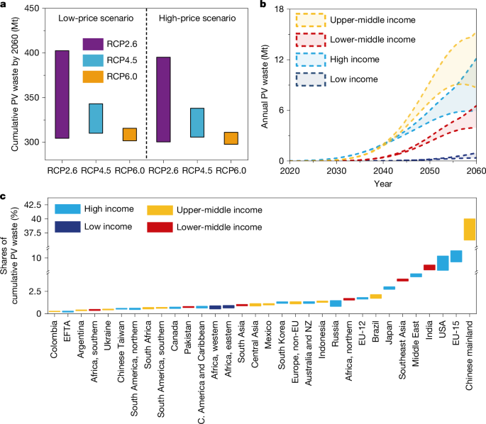
Here we develop an integrated modelling framework to project PV waste generation across 32 global regions and to quantify the environmental and economic benefits of alternative recycling strategies that will inform policy design (Extended Data Fig. 1 and Supplementary Table 3). The framework consists of three interconnected components. First, material price trajectories are generated and incorporated into the GCAM to simulate regional PV deployment under alternative socioeconomic–climate futures. GCAM electricity-generation outputs are then converted into installed PV capacity and passed to a dynamic material flow analysis to estimate regional EOL PV waste. Second, projected waste streams are coupled with life-cycle assessment (LCA) and life cycle cost (LCC) to quantify technology-specific economic and climate outcomes of PV recycling. Third, a multidimensional scenario design, covering decommissioning pathways, recycling technologies, international trade configurations and subsidy schemes, is applied across the modelling system to assess how policy and market structures reshape regional recycling outcomes. Detailed parameter settings are provided in Supplementary Tables 4–9.

Material price model

To account for the impact of price uncertainty of critical materials on PV recycling, we simulate long-term price trajectories for four solar-relevant critical materials: copper, aluminium, silver and silicon. We adopt a material price model that was developed in previous studies^7,51,52, incorporating historical price dynamics, demand growth and substitution potential. The resulting price trajectories are then introduced as exogenous inputs into the GCAM to determine PV deployment pathways under climate targets (as detailed in the next section). Rather than generating precise forecasts of future prices, our objective is to construct scenario-based price trajectories that enable the evaluation of PV deployment and recycling pathways under long-term material price uncertainty.

The material price model is grounded in dynamic market equilibrium in which long-term prices are endogenously determined by the marginal cost of new supply required to meet future demand. When existing mining capacity is insufficient, additional mining projects must be operated. Material prices are therefore endogenously governed by the marginal cost of newly installed mining capacity.

The modelling procedure consists of three steps:

Step 1: demand projection. Future demand for critical materials is determined by the demand growth rate and price-responsive substitution effects:

where Q^t denotes the material demand in period t; g is the annual exogenous demand growth rate (Supplementary Table 4); ε is the price elasticity of demand; and Δp^t is the annual price change rate in period t, defined as

The initial price p₀ is exogenously specified use the global average price for each material in 2020.

Step 2: new capacity requirement and price determination. The required new mining capacity to meet the future demand is calculated as:

where O^t+1 denotes the newly required annual production capacity in period t + 1; L^t represents supply losses from mine closures due to resource depletion in period t and R^t is the secondary supply in period t.

The marginal cost of new mining capacity in period t (I^t) is determined using an incentive cost curve:

where a^t represents the minimum marginal cost of new mining capacity in period t and b^t captures the rate at which marginal costs increase in period t due to factors such as declining ore grade and more complex investment conditions. The equilibrium material price in year t is therefore determined by the most expensive marginal cost of the required new capacity:

Step 3: evolution of mining cost structure. The incentive cost curve evolves over time due to ore grade depletion, technological progress and changes in operating costs⁵¹. We introduce a cost-adjustment factor n to capture these dynamics:

where e is the annual growth rate of operating costs (for example, energy, labour, water, reagents, environmental compliance); t_g represents annual cost reduction rates from technological progress; and l is the annual ore-grade depletion rate.

The intercept of the operating mine cost curve (a^t+1) is updated as the minimum of two factors: (1) the cheapest operating mine cost in the last period t adjusted by n_t and (2) the operating cost of the cheapest mine that newly opened in the current period (t + 1) (after subtracting annualized capital cost c_a):

The upper bound of the operating curve C^t+1(1), which represents the operating cost of the most expensive active mine in the period t + 1, is updated as

This formulation follows two mechanisms: (1) mines with operating costs exceeding the previous period’s market price (p^t) are assumed to exit the market, and (2) new mines enter the market only if their operating costs are covered by the current material price net of annualized capital cost (p^t+1 − c_a). Taking the maximum of these two values ensures that the operating cost frontier is consistent with both the exit of unprofitable existing mines and the entry condition for new capacity.

The slope of the operating cost curve is then updated as

Further details of the model structure and assumptions can be found in our previous paper⁷.

Material price scenarios

To characterize long-term uncertainty in critical material prices and its impacts on global PV deployment and decommissioning, we construct alternative price scenarios within the material price modelling framework. Scenario variation is introduced by varying parameters that reflect (1) technological progress in mining productivity and (2) material substitution potential. Improvements in mining productivity are represented as t_g − e, which is the difference between the reduction in mining costs due to technological progress (t_g) and the increases in operating cost (e) (see Eq. 6). Material substitution is captured by the price elasticity parameter ε in equation (1), which reflects the responsiveness of demand to price changes through substitution toward alternative materials.

These parameters take values within the ranges reported in the literature, and details are provided in Supplementary Table 4. For both mining productivity and substitution elasticity, we classify parameter values into low and high categories using the midpoint of each reported range as the threshold. Combining these assumptions yields two contrasting price scenarios that span plausible bounds of long-run material price uncertainty:

1. (1)

   Low-price scenario: assumes strong technological progress in both mining productivity (resulting in fast mining cost reductions and declining operating costs) and material substitution capabilities, thereby moderating future price increase.

2. (2)

   High-price scenario: assumes limited technological advancement in mining productivity and weak material substitution potential, resulting in tighter supply conditions and higher long-run prices.

Under these scenario settings, the price trajectories for four solar-relevant critical materials (copper, aluminium, silver and silicon) are simulated. Extended Data Fig. 2 illustrates the projected price pathways under the two scenario settings.

GCAM model

The GCAM is an integrated assessment model that links five interconnected systems: water, energy, land use, socioeconomics and climate. It is a common model that has been used in international and national scenario assessments^52,53. GCAM represents a broad portfolio of electricity generation technologies, including solar photovoltaics and wind power. Renewable resources are assumed to be region-specific and non-tradable across regions. Technology deployment is determined through an internally consistent, multistage process that links technology costs, resource supply curves and market-based technology choice.

From capital cost to electricity generation in GCAM

Incorporating material price shocks into capital costs

To quantify the effect of critical material price increases on the deployment of solar PV, simulated material price trajectories are translated into technology-specific capital cost changes under price scenarios. The capital cost of solar PV in the year t is defined as

where \({C}_{\text{BLS},t}\) is the baseline capital cost of PV following GCAM’s default setting⁵⁴ and ΔC_t represents the change of cost increment induced by material price changes:

where MI_m is the material intensity of material m in solar PV, P_mt is the simulated material price under alternative price scenarios in year t, and \({P}_{mt,\mathrm{BLS}}\) is the corresponding baseline material price.

Total technology cost

The total cost of electricity generation technology in GCAM is calculated as⁷

where t(C_t) represents capital and fixed operating costs; p_j is the marginal cost of input resource j; gk is the cost associated with emissions of greenhouse gas k; and v_l is the value of secondary outputs. For solar technologies, p_j is determined through the renewable resource supply curve Q (equation (15)).

Technology choice and market shares

Technology shares in electricity generation are determined using a relative-cost logit formulation in GCAM⁷. The share of generation technology j is calculated as

where α_j is a technology-specific share weight, C_total,j is the total cost of technology j, and γ is the logit exponent controlling the sensitivity of technology shares to cost differences. Technologies with lower relative costs gain larger market shares.

The electricity generation Q^e from technology j is then given by:

where D is the total electricity demand under a given SSP.

Renewable resource supply curves

To capture spatial and technological heterogeneity in renewable resource availability, GCAM uses region- and technology-specific resource supply curves. The cumulative generation potential available at or below a given marginal cost p is defined as⁷

where MaxSubResource represents the maximum exploitable resource potential, MidPrice is the cost at which half of this potential becomes available, and curveExponent is the steepness of the supply curve.

For PV, GCAM assumes an effectively flat and abundant resource base, reflecting high solar potential in many regions and the modular scalability of PV systems. Under this assumption, marginal resource costs do not increase with deployment, allowing material price shocks to transmit primarily through capital costs.

To ensure the accuracy of historical data and the model’s backcasting capability, we cross-validated the historical electricity generation outputs from GCAM against IRENA’s official statistics; detailed comparisons are provided in Supplementary Note 1 and Supplementary Fig. 3.

From electricity generation to installed capacity

To estimate solar PV waste, electricity generation outputs from GCAM are converted into installed capacity. As GCAM reports generation in exajoules (EJ), values are first converted to gigawatt-hours (GW h) using a constant conversion factor (ω = 277,778.8). Installed capacity is then derived by dividing annual electricity generation by the product of annual operating hours (T = 8,760) and the capacity factor^7,55:

where \({\mathrm{IC}}_{i,t}\) is the installed capacity (GW) in region i and year t; EJ_i,t represents the annual electricity generation (EJ) for region i in year t; and CF_i denotes the region-specific capacity factor.

Integrated socioeconomic–climate scenarios

The GCAM generates internally consistent energy–economy–land–climate pathways under alternative socioeconomic and climate policy assumptions. In this study, we couple five SSPs (SSP1–SSP5) with three Representative Concentration Pathways (RCP2.6, RCP4.5 and RCP6.0) to construct a comprehensive set of socioeconomic–climate scenarios for evaluating future PV deployment⁵³. For presentation purposes only, these combinations are classified into frequently used benchmark pathways and supplementary stress-test pathways according to their prevalence in the literature⁵⁶. This classification does not alter model simulations or parameterization. The full classification and detailed descriptions of scenarios are provided in Supplementary Table 3, with further discussion on specific scenarios in Supplementary Note 2. All simulations are conducted using GCAM v.8.2. For each scenario, we extract regional solar electricity generation trajectories and subsequently aggregate GCAM regions into four income groups (Supplementary Table 1). Detailed documentation of the model structure and assumptions is available in the GCAM v.8.2 Documentation: GCAM Model Overview, accessible at https://jgcri.github.io/gcam-doc/overview.html.

Projection of future PV waste generation

Future PV waste generation is estimated using a dynamic MFA model. MFA is extensively used to quantify the evolution of material stocks and flows over time, including the estimation of waste streams from solar energy systems^57,58. A key input to the MFA model is annual PV in-use capacity, comprising historical installed capacity and projected additions. Historical installed capacity for 2000–2024 is updated using the 2025 statistics from the IRENA⁵⁹ (Supplementary Tables 10–13). Extending the time series to 2000 enables calibration of early decommissioning volumes. The primary analytical period reported in the main results is 2020–2060. Future PV capacity trajectories are derived from GCAM projections at five-year intervals and interpolated to annual values using cubic spline interpolation to estimate newly added capacity. The estimation is then performed in two steps: (1) calculating annual inflows and outflows of PV capacity; and (2) converting decommissioned capacity into waste mass.

Step 1: PV capacity inflow and outflow are determined using a Weibull lifetime distribution⁵⁸:

where t denotes year (2000–2060), t′ is the installation year of the PV panel, and t − t′ represents the service time of the panel. F(t − t′) is the cumulative Weibull distribution function. T is the average lifetime of PV panels (30 years), and β is the shape parameter. A regular-loss scheme is adopted, assuming no premature loss over the module lifetime. Under this assumption, the Weibull shape parameter is set to β = 5.3759 (ref. ⁶⁰). The quantities outflow_i(t), stock_i(t) and inflow_i(t) denote decommission capacity, in-use capacity and newly added capacity for region i in year t, respectively. The initial stock is assumed equal to the first-year inflow.

Step 2: decommissioned capacity is converted to waste mass PVWaste_i(t) using timing-varying weight-to-power ratios perPVton(t) (refs. ^26,57):

where perPVton(t) denotes the PV module weight-to-power ratio for period t, obtained from IRENA reports⁶⁰ (Supplementary Table 14). As projections in IRENA reports are available only until 2050 (ref. ⁶⁰), the 2050 ratio is assumed constant thereafter. Annual inflow, annual outflow and in-use stock trajectories for 2020–2060 are presented in Supplementary Figs. 4–6. The analysis focuses exclusively on crystalline-silicon (c-Si) PV modules, which have accounted for more than 90% of global PV installations since 2012 (ref. ⁶¹); other PV technologies are therefore excluded. Detailed assumptions are described in Supplementary Note 3.1.

Economic cost–benefit analysis

The economic feasibility of recycling EOL PV panels is evaluated using an LCC framework, which is consistent with the LCA system boundary and quantifies the economic costs and benefits associated with recycling PV modules over their entire life cycle^23,62. Recycling costs are first estimated for the base year (2020) at the unit level (that is, US$ per tonne of PV waste), then adjusted dynamically to reflect technological learning and scale effects, and finally multiplied by projected regional PV waste volumes to estimate total economic costs. Economic benefits are calculated based on the market value of recovered secondary materials. The detailed calculation steps are presented as follows.

The unit total costs, uTC, of PV waste recycling comprises stage-specific costs and whole-process costs. Stage-specific costs are variable expenditures incurred at each processing stage, whereas whole-process costs refer to overhead expenditures spanning the entire recycling chain.

The base year (2020) unit total recycling cost (uTC₀) is calculated as follows⁶²:

where uC_ss represents the stage-specific unit costs for collection (ss = 1), transportation (ss = 2), dismantling (ss = 3), technical treatment (ss = 4) and disposal (ss = 5). uC_w denotes the whole-process unit costs, including labour (uC_l), management (uC_m), depreciation of fixed assets (uC_f), operation and maintenance (uC_ope), and opportunity costs (uC_opp).

Owing to the limited global data on differentiated recycling costs, we adopted a comprehensive, internally consistent cost-benefit inventory for China from our previous study⁵⁶ as the reference baseline. Except for region-specific labour, collection, and transportation costs, other unit cost components (such as technical treatment, dismantling and operational expenses) are extrapolated to region iusing purchasing power parity (PPP) adjustments (detailed descriptions of the assumptions are provided in Supplementary Note 3.2):

where uC_i,0 is the estimated unit cost for region i in the base year 2020, uC_CN,0 is the 2020 baseline cost in China, PPP_CN,0 and PPP_i,0, respectively, represent the PPP conversion factors in China and region i in 2020, and ER_i,0 denotes the market exchange rate of region i in 2020 (Supplementary Table 15).

Region-specific collection costs are determined following previous study⁶³. Labour costs are estimated based on national per capita gross national income (GNI) data from the United Nations Trade and Development Data Hub⁶⁴, assuming a per capita PV recycling capacity of 100 tonnes per year⁶². Transportation costs include domestic and international maritime transport. Domestic maritime costs are calculated following equation (23) due to limited national level data. International maritime transport costs are estimated based on bilateral maritime distances and a unit sea freight cost of US$0.1 per nautical mile per twenty-foot equivalent unit⁶⁵, assuming a maximum capacity of 30 t per container following ISO standards⁶⁶. Bilateral maritime distances are derived from a global port network approach^67,68. Shortest port-to-port navigable maritime routes are computed for all possible pairs between trading regions, rather than relying on spherical distances between national centroids. To avoid bias from exceptionally short routes, the 10th percentile of the resulting route-distance distribution is adopted as the representative bilateral shipping distance for each region pair. Given that the shortest port-to-port distances often underestimate actual maritime routes, a correction factor of 1.3 is applied to approximate real-world sailing conditions⁶⁷. Region-level costs are then aggregated to the 32 GCAM regions using arithmetic means. Regional base-year (2020) unit costs are illustrated in Extended Data Fig. 9.

It is expected that unit recycling costs of PV waste will decrease over time as a result of technological learning and scale expansion, adhering to the learning curve principle^23,43. To account for irreducible production inputs that limit cost reductions, we use a modified learning curve formulation with an irreducible cost floor⁵⁴:

where uTC_t denotes the unit recycling cost in year t and uTC₀ denotes the initial cost in 2020. t₀ is the base year (2020) and LR is the learning rate. The learning rate values are derived from previous studies^23,69,70. Detailed descriptions of the assumptions regarding learning rate can be found in Supplementary Note 3.3. The parameter C_{min_ratio} represents the minimum cost coefficient reflecting irreducible production inputs, such as energy consumption, chemical reagents and base labour, that cannot be entirely eliminated through learning. Based on the evidence that global PV costs declined by up to 87% between 2010 and 2024 (ref. ⁷¹), we set C_{min_ratio} to 0.13, implying an asymptotic lower bound of C₀ × C_{min_ratio}, with an assumption that recycling cost will follow a similar trajectory.

Total recycling cost (TC_t) in year t is calculated as the product of the dynamically adjusted unit recycling cost (uTC_t) and the total PV waste volume (PVWaste_t):

where π denotes the assumed annual inflation rate calibrated based on the global average inflation rate over 2000–2024 (ref. ⁷²).

Total recycling benefits in year t (B_t) are derived from the market value of recovered secondary materials, including aluminium, glass, silver, copper and silicon^73,74. It depends on material prices, recovery efficiencies and decommissioned PV volumes. Material prices are set to correspond with different material price escalation scenarios to reflect potential resource scarcity and market volatility (Extended Data Fig. 2 and Supplementary Fig. 1). Total benefits are calculated as

where P_mt is the simulated price of material m under alternative price scenarios in year t and uR_m denotes the unit recovery quantity (Supplementary Tables 16–18). All unit costs and material prices are first projected in constant 2020 US$. Nominal values are subsequently derived by applying an inflation factor.

The nominal net economic benefit (NB_t) and the unit nominal net benefit (UNB_t) are calculated as:

Detailed data and accounting procedures for unit costs and benefits are provided in our previous paper⁶².

Climate benefits from PV recycling

We quantify the climate benefit of PV module recycling as the net avoided greenhouse gas (GHG) emissions (in CO₂ equiv.) generated by recycling 1 t of EOL c-Si PV panels:

where CB_s,i,c,t denotes the net climate benefit of recycling technology s in region i under climate pathway c in year t; RB_s,i,c,t represents the recycling benefit (avoided GHG) generated during recycling; and RG_s,i,c,t denotes GHG emissions released during the recycling process. The recycling benefit RB_s,i,c,t comprises two components: one is that recovered materials substitute for virgin materials of equivalent quality and quantity, thereby avoiding emissions from primary extraction, refining and manufacturing of virgin PV materials^21,75, the other is that, where applicable, energy recovery from polymeric fractions (for example, backsheets and encapsulants) offsets emissions that would otherwise arise from conventional energy supply⁶². The recycling burdens RG_s,i,c,t includes all emissions generated throughout the EOL treatment chain, covering electricity use, auxiliary inputs and transportation of waste modules, intermediate fractions and residual wastes^76,77.

Following the life-cycle assessment framework^62,78, the functional unit is defined as 1 t of EOL c-Si PV panels. The system boundary from collecting PV module wastes to recovering secondary materials and energy is shown in Supplementary Fig. 7.

Note that the GHG emission intensity of electricity generation evolves over time under different climate policy pathways and varies substantially across regions. To account for this heterogeneity, we adjust the electricity-related emission intensity in the LCA framework using region-, pathway- and year-specific electricity-sector emission factors. The actual electricity emission factor is defined as

where EF_i,c,t is the electricity-sector emission factor in region i under climate pathway c in year t; EF_i,c,base is the base year (2020) emission factor; and α_i,c,t is the adjustment coefficient that captures deviations from the baseline electricity emission intensity. Therefore, the final climate benefit of PV recycling is

where \({\mathrm{RB}}_{s}^{\mathrm{elec}}\) and \({\mathrm{RB}}_{s}^{\text{non-elec}}\) represent the electricity-related and non-electricity-related recycling benefits, respectively, under base-year electricity emission factors for recycling technology s. \({\mathrm{RC}}_{s}^{\mathrm{elec}}\) and \({\mathrm{RC}}_{s}^{\text{non-elec}}\) denote the electricity-related and non-electricity-related recycling burdens associated with the recycling process.

Given that carbon dioxide accounts for more than 70% of total GHG emissions⁷⁹ and constitutes the primary contributor to the global warming potential (GWP) of PV recycling, mainly due to transport-related fuel consumption, polymer incineration and coal-based electricity generation^38,77,78, this study assumes that the temporal evolution of regional GHG emission factors is consistent with the carbon emission trajectories projected by GCAM (Supplementary Fig. 8). Detailed process inventories are reported in Supplementary Tables 16–18 and described in ref. ⁶².

Recycling technology scenarios

To capture the dynamic evolution of PV recycling technologies across regions and over time, we developed an integrated framework combining scenario design, a Logit-based technology choice model and region-specific heterogeneity constraints⁸⁰. The framework explicitly accounts for cross-regional differences in low-carbon technologies investment, technological capacity, environmental regulation stringency and projected PV waste generation, all of which collectively determine feasible recycling technology mixes. The mechanical, thermal and chemical recycling technologies coexist and compete, with market shares evolving endogenously under heterogeneous regional conditions.

Based on this framework, four recycling technology scenarios are constructed: BAU, economic-priority, carbon-priority and technology diffusion.

Under the BAU scenario, the recycling technology structure in each region is assumed to remain constant throughout the study period. Technology market shares are fixed at base-year (2020) levels and do not respond to changes in economic performance or climate benefits. Base-year shares are calibrated using information on recycling patent distributions and facility locations reported by IEA³¹ (Supplementary Tables 19 and 20), reflecting existing technological endowments and path dependency across regions.

Under the economic-priority scenario, recycling technology choices are driven primarily by economic rationality. The attractiveness of each technology is determined by its net economic benefit, the difference between revenues from recovered secondary materials and associated recycling costs. Technology market shares evolve endogenously in response to relative net profits, capturing competitive dynamics among alternative recycling options under profit-oriented decision-making. However, the evolution of clean and low-carbon technologies is also shaped by regional disparities in investment capacity. As noted in previous studies^81,82,83, investment in low-carbon technologies and related R&D remains concentrated in developed regions. Most emerging markets and developing regions have limited access to these technologies owing to constrained investment capabilities, and therefore continue to rely on existing technologies, experiencing slower rates of technological upgrading. Consequently, under this scenario, mechanical recycling, which is less capital-intensive but exhibits lower recovery efficiency for high-value metals and therefore generates smaller net profits per unit of waste recycled than the other two technologies, captures a larger market share in many middle- and low-income regions. Moreover, its market share declines more slowly in these regions than in high-income regions.

The carbon-priority scenario represents a climate-driven decision framework in which technology attractiveness is determined by carbon mitigation performance. Specifically, the choice variable is defined as the carbon reduction benefit of PV waste recycling, measured as avoided GHG (for example, kg CO₂ equiv.). To capture cross-regional differences in regulatory ambition and policy enforcement, region-specific parameters (climate policy stringency index) are introduced based on the OECD Environmental Policy Stringency Index⁸⁴. Higher policy stringency drives technology evolution towards technologies with the greatest carbon mitigation benefits.

The technology diffusion scenario is designed by analogy with historical PV patent diffusion patterns observed between 1970 and 2022. Given the projected sharp increase in PV waste generation after 2040 (ref. ⁵⁸), recycling technology diffusion is modelled as a staged process comprising four phases: before 2030, technology shares remain at baseline levels; 2030–2040 represents an early adoption phase, analogous to the 1970–2000 PV patent diffusion period; 2040–2050 corresponds to an accelerated expansion phase, reflecting the 2001–2011 period; and 2050–2060 represents a maturation phase, similar to 2012–2022. Recipient regions are assumed to gradually converge toward the technology structures of leading regions as diffusion progresses. Stage-specific diffusion parameters are calibrated based on historical PV patent data reported in a previous study⁸⁵. Detailed descriptions of the assumptions are provided in Supplementary Note 3.4.

Logit-based technology choice model

In the economic-priority and carbon-priority scenarios, recycling technology market shares are determined using a logit-based choice model that allows multiple technologies to coexist and compete within each region⁸⁰.

For each region i and time t, technology market shares satisfy the adding-up constraint:

where s index recycling technologies (mechanical, thermal and chemical recycling technologies).

The market share of technology s in region i at time t, denoted as \({\mathrm{Share}}_{s,i,t}\), is given by

where P_s,i represents the base-year (2020) weight of technology s in region i, capturing existing infrastructure and path dependency; V_s,i,t denotes the scenario-specific performance indicator, defined as the net economic benefit in the economic-priority scenario and the carbon reduction benefit in the carbon-priority scenario; and γ_i is a region-specific parameter representing the investment capacity index for low-carbon technologies under the economic-priority scenario, or the climate policy stringency index under the carbon-priority scenario, where larger values indicate a stronger concentration of market shares toward the best-performing technology (Supplementary Table 21).

Recycling trade scenarios

Current strategies for managing EOL PV modules generally fall into two categories: domestic recycling and outsourced recycling. In some regions, such as the EU and South Korea, regulatory frameworks based on the principle of EPR¹⁰ require manufacturers to take responsibility for the collection, transport, and recycling of decommissioned PV modules. Meanwhile, the globalization of PV supply chains, where 76.89% of newly installed capacity in 2017 involved imported modules⁸⁶, suggests that future EOL management may increasingly transcend national boundaries. Consequently, cross-border waste trade is likely to become a structural feature of global EOL PV management, particularly for regions that have relied heavily on imported modules without developing corresponding domestic recycling capacity.

PV recycling capabilities are unevenly distributed worldwide. Only a limited number of regions, including China, the United States, the EU, Japan and South Korea, possess mature infrastructure and patented technologies necessary for formal recycling processes⁸⁷. By contrast, many regions in the Global South face considerable constraints related to limited industrial capacity, lack of technical expertise and weak regulatory enforcement^41,88. In such contexts, EOL PV modules may either be exported to technologically advanced regions or processed through informal recycling sectors⁴⁰, which often operate outside regulatory oversight and may entail environmental and health risks⁸⁸.

To examine how alternative international cooperation structures influence climate and economic outcomes, four recycling trade scenarios are constructed: local recycling, extended producer-responsibility-oriented trade, expanded global trade and regional trade. These scenarios reflect varying degrees of domestic versus outsourced recycling, informed by trade data, policy frameworks and access to technology. In this study, the term transboundary flow refers specifically to the international shipment of intact EOL PV modules. The underlying assumptions and rationale are described in Supplementary Note 3.5.

Under the local recycling scenario, regions with established PV recycling technologies are assumed to process 100% of their domestically generated EOL modules within national borders, and international trade in PV waste is not permitted. Regions without recycling technologies are assumed unable to recycle, resulting in zero recycling benefits. This scenario serves as a benchmark for isolating the role of domestic recycling capacity and for evaluating the economic, climate and equality implications of international trade.

The extended producer responsibility–oriented trade scenario reflects an international recycling system governed by EPR principles. EOL PV modules are exported back to the regions or regions responsible for their original production (a return-to-producer rule), following historical bilateral PV module trade routes, consistent with scenario assumptions adopted in previous studies⁸⁶. Recycling activities are conducted in PV producer (exporting) regions, which bear the associated treatment costs while retaining revenues from recovered secondary materials. Historical trade structures are assumed to remain fixed through 2060. This scenario represents a regulatory-driven recycling framework emphasizing producer accountability and path dependence. The PV module trade data are adopted from a previously published study⁸⁶. Extended Data Fig. 8 illustrates the geographical distribution and allocation patterns of waste flows under various trade scenarios.

The expanded global trade scenario represents a highly integrated international recycling system in which all regions with PV recycling technologies are eligible to act as waste importers. Regions without recycling technologies must export their EOL PV modules to recycling-capable regions. The allocation of exported waste across eligible importing regions is determined by a composite weighting scheme based on economic globalization and trade openness indices derived from established datasets⁸⁹ (Supplementary Table 22). Regions with higher index values receive larger shares of imported PV waste, reflecting lower trade barriers, stronger logistics capacity and greater institutional readiness for cross-border material circulation. Trade structures are assumed to be constant through 2060. The underlying assumptions and rationale are detailed in Supplementary Note 3.6.

The regional trade scenario constrains international PV waste trade within geographically defined continental regions, disallowing intercontinental trade. Following the United Nations’ geographical classification, all regions are grouped into five continental regions: Africa, Asia, Europe, the Americas and Oceania. Within each region, regions without recycling technologies export EOL PV modules to recycling-capable regions in the same region. As in the expanded global trade scenario, the distribution of waste among eligible importers is determined by relative economic globalization and trade openness indices, calculated at the regional level. This scenario represents a geographically bounded form of international cooperation, reflecting potential logistical, regulatory and political constraints on intercontinental waste transport. Trade structures are likewise assumed to remain constant through 2060 (ref. ⁸⁶).

Variance analysis of recycling benefits

To evaluate how recycling trade scenarios impact PV recycling equality, we use the cross-regional dispersion of realized recycling benefits as a transparent and comparable proxy for distributional equality. Specifically, for each scenario j, we calculate the variance of regional benefits across the 32 modelled regions. The variance \({\sigma }_{\mathrm{sc}}^{2}\) is computed as

where EB_i,sc represents the recycling-related benefit (economic or climate) of region i under scenario sc and \(\overline{{\mathrm{EB}}_{\mathrm{sc}}}\) denotes the corresponding mean benefit across all n = 32 regions. A larger variance indicates greater dispersion in realized benefits and thus a more unequal distribution across regions.

To facilitate comparison across scenarios with potentially different absolute dispersion levels, variances are normalized to the range [0, 1] using min–max normalization:

where \({\sigma }_{\min }^{2}\) and \({\sigma }_{\max }^{2}\), respectively, represent the minimum and maximum variance values across all scenarios. The normalized variance \({\sigma }_{\mathrm{sc}}^{2* }\) reflects the relative inequality level of each scenario: 0 corresponds to the most equitable distribution (lowest variance) and 1 corresponds to the most unequal distribution (maximal variance).

Note that this variance-based indicator captures disparities in realized economic and climate benefits across regions under each scenario without accounting for procedural equity or environmental justice. In this context, the metric serves as a descriptive and comparable measure of distributional dispersion.

Subsidy scenarios

To encourage participation in PV waste recycling and mitigate the risk of excessive spatial concentration of recycling activities, we developed a set of alternative recycling subsidy scenarios. These scenarios represent policy instruments widely discussed in PV and electronic waste recycling literature, and capture both direct fiscal interventions and market-based environmental incentives^73,90,91,92.

Five subsidy scenarios are considered: (1) no subsidy; (2) continuous subsidy; (3) declining subsidy; (4) low-carbon price; and (5) high-carbon price. No subsidy represents a reference scenario where recycling operations receive no direct fiscal support or carbon price-based financial incentives. The continuous subsidy and declining subsidy scenarios represent cost-based fiscal interventions that reduce the effective cost of recycling, while the latter two represent market-based environmental incentives linked to avoided carbon emissions. Scenario design and parameter ranges are informed by existing policy documents and previous studies on recycling and circular economy policies^{43,90,91,92,93,94}.

Cost-based subsidy scenarios

The continuous subsidy scenario reflects sustained fiscal support throughout the project lifetime, consistent with recent circular economy policy frameworks⁹². Under this scenario, governments provide an annual subsidy proportional to total recycling costs, including both capital expenditure (CapEx) and operating expenditure (OpEx). The annual subsidy for region i in year t is expressed as

where \({\mathrm{TC}}_{i,t}^{\mathrm{total}}\) denotes the total recycling cost in region i and year t and \({w}_{i,t}\) represents the subsidy rate. Owing to the limited region-specific policies and substantial uncertainty regarding appropriate subsidy magnitudes, subsidy rates were sampled from a range of 0–15%, consistent with the upper bound observed in existing circular economy investment programs⁹². Both cost-based subsidy scenarios are evaluated using 1,000 Monte Carlo simulations to reflect this uncertainty.

The declining subsidy scenario represents a transitional support mechanism in which subsidies are gradually withdrawn as recycling activities become economically viable⁹⁰. Subsidies are initially applied at the same rate as in the continuous subsidy scenario, but decline annually by a fixed proportion δ once recycling becomes economically variable until it fully phases out. Break-even is defined as the first year when annual net recycling revenue in region i becomes non-negative. This declining subsidy is formulated as

where δ = 0.10 represents the annual reduction rate of the subsidy after break-even, \({t}_{i}^{* }\) denotes the break-even year, and \({w}_{i,0}\) denotes the subsidy rate in the base year (2020) in region i.

Carbon-price-based subsidy scenarios

The low-carbon-price and high-carbon-price scenarios are derived from two policy pathways proposed by the International Energy Agency⁹⁵: the Stated Policies Scenario (STEPS) and the Announced Pledges Scenario (APS), respectively. In the high-carbon price scenario, regions that have committed to net-zero emission targets adopt carbon prices consistent with the APS pathway over time. By contrast, the low-carbon-price scenario applies carbon prices equivalent to 30–80% of the APS levels and only to regions that have implemented, or formally announced plans to implement carbon pricing mechanisms (for example, Canada, South Korea, China and the EU).

Under these scenarios, recycling subsidies are proportional to avoided carbon emissions from PV module recycling. The annual carbon-related subsidy received by region i in year t is calculated as

where \({P}_{i,t}^{\text{C}{{\rm{O}}}_{2}}\) denotes the region-specific carbon price in region i and year t and \({\mathrm{TEI}}_{i,t}\) represents the avoided carbon emissions resulting from PV recycling activities in region i and year t. Carbon price data for 2030 and previous years were obtained from the World Bank report⁹⁶. Carbon price data after 2030 were sourced from the International Energy Agency⁹⁵.

Incorporation of subsidies into net benefits

Across all scenarios, subsidies are incorporated into the annual net benefit (NB) calculation either as a reduction in effective recycling costs (cost-based subsidy scenarios) or as an additional revenue (carbon-price based subsidy scenarios). The annual net benefit for region i in year t is calculated as

where \({B}_{i,t,\mathrm{sc}}^{\mathrm{total}}\) denotes the revenue from recovered materials in region i and year t under a given scenario sc, S_i,t,sc represents the subsidy received in region i and year t under a given scenario sc and \({{\rm{TC}}}_{i,t,\mathrm{sc}}^{\mathrm{total}}\) is the total recycling cost in region i and year t under a given scenario sc, including both capital and operating expenditures.

Equality evaluation of subsidy effects

To evaluate how subsidy policies affect regional disparities in recycling benefits, we quantify inequality in unit net recycling benefits across the 32 regions using two complementary indicators: (1) variance (dispersion) and (2) maximum-minimum benefit gaps (extreme disparity), and compare pre- and post-subsidy indicators. Both indicators are calculated for each scenario sc and year t, before and after subsidy implementation.

The pre-subsidy variance of unit net benefits is calculated as

where UNB_i,sc,t denotes the unit net recycling benefit in region i under scenario sc in year t before subsidies, \({\bar{\mathrm{UNB}}}_{\mathrm{sc},t}\) is the corresponding regional mean and N is the number of regions (N = 32).

After subsidy implementation, unit net benefits are recalculated as

and the post-subsidy variance becomes

where \({\overline{\mathrm{SUB}\_\mathrm{UNB}}}_{\mathrm{sc},t}\) represents the mean unit net benefit across regions under scenario sc in year t after subsidies.

To capture extreme disparities, we computed the net unit recycling benefit gaps for scenario sc in year t as

where \({\mathrm{Gap}}_{\mathrm{sc},t}^{\mathrm{pre}}\) and \({\mathrm{Gap}}_{\mathrm{sc},t}^{\mathrm{post}}\) denote the net unit recycling benefit gaps before and after the implementation of subsidies, respectively, in scenario sc and year t.

Uncertainty analysis

To assess the robustness of the modelling results and core conclusions, we conducted a series of uncertainty and sensitivity analyses (Supplementary Note 4, Supplementary Table 23 and Supplementary Fig. 9), focusing on PV module lifetime, material intensity, inflation rates and carbon price parameters. First, alternative lifetime extensions and reductions in material intensity were implemented to reflect potential technological progress. The results indicate that each of these measures can substantially reduce future PV waste generation. Second, we evaluated the impact of macroeconomic uncertainty by testing alternative high- and low-inflation trajectories and recalculating net economic benefits of PV recycling. Across these scenarios, variations in inflation rates exert only a limited influence on estimated net benefits. Third, we evaluated the sensitivity of distributional outcomes to alternative carbon price growth trajectories during 2050–2060, particularly under high carbon-price subsidy assumptions. The results show that even under alternative carbon price growth rates, high carbon prices consistently exacerbate inequalities in recycling benefits across regions, confirming the robustness of our findings.

Reporting summary

Further information on research design is available in the Nature Portfolio Reporting Summary linked to this article.